Figure 1. There is steady high rate of glitches in the mid-frequency band. I do not remember seeing such an issue in the past few years. It is possible that will resolve itself as the adjustment of the interferometer thermal compensation and controls are in progress, but it is not likely. Starting investigating what are the properties of these glitches should start in parallel of the on-going interferometer tuning.
FWIW, online Bruco wasn't able to run overnight as it didn't find any long enough segment w/o strong glitch.
Daily UPV finds some SDB1 witness channels but they only account for a few percents of those glitches.
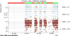
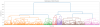
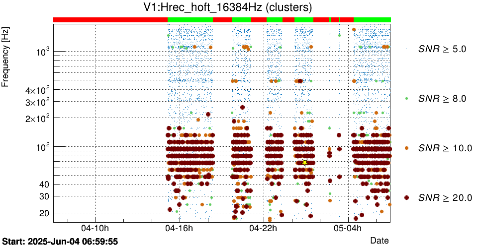
I've hacked a Virgo DQR script to zoom onto those glitches over a few minutes -- see plot in attachment
- Top: the Omicron triggers (before time clustering)
- Middle: the standard Omicron clusters (after time clustering; what we usually call Omicron "triggers")
- Bottom: an attempt to make 2D (time-frequency) clusters
=> Most of the strong glitches (dark brown) are short in time and very wide in frequency.
I tried to investigate the correlation between these glitches and the auxiliary channels. First, I identified a BRMS channel from Hrec that could serve as a glitch witness: V1:DQ_BRMSMonHrec_BRMS_HREC_HOFT_FREQ_BAND_85_95_Hrec_hoft_16384Hz seemed like a reasonable choice. I then computed correlations with all _mean and _rms trend channels, as described in a previous entry (#66922).
Fairly high correlations were found with the following channels V1:Sc_WI_FF50HZ_*_rms, and V1:Sc_BS_CMRF_rms V1:SDB2_POWERSUPPLY_DBOX_LEFT_DOWN_p12V_rms.
One possibility is that the observed correlations arise from these channels "reacting" to the loud glitches in the strain channel, rather than being causally related to their origin. Therefore, this study does not appear to provide new insights into the origin of these glitches.
As with the range correlation study (#66922), more information may become available once we have access to longer stretches of undisturbed data in DQ Studies operational mode.
Analyzing Saturday's data, Online BruCo found a single segment "clean" enough to process it. The corresponding GPS range is 1433330363 (Jun 07, 2025 11:19:05 UTC) -> 1433331348 (Jun 07, 2025 11:35:30 UTC); but looking at the corresponding Omicron plots, that looks more a temporary downwards fluctuation of the glitch rate below the BruCo threshold than a significant variation of the glitch pattern.
Looking at the automatic UPV report over the last week, 2 channels witness the excess of glitches in h(t): SDB1_OMC1_Peltier_cmd and SDB1_OMC1_err. This is not a 100% match: about 5% of glitches are found in coincidence with glitches in OMC channels. Maybe this is a hint about where to look... Experts will know.
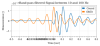
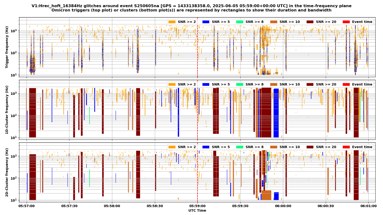
Figure 1. Looking at the UPV report, about 50% of the glitches with SNR greater than 100 are caught by these channels based on the OMC error signal. With the exception of the peak at SNR ~400 that probably correspond to the 25 minute glitches.
The high efficiency of vetoing very loud glitches in h(t) based on the OMC error signal is not informative. The OMC error signal is based on the same photodiode as h(t), the only difference is that it is demodulated at 12.8kHz. For a loud enough glitch at ~100Hz it will also disturb the demodulation at 12.8kHz and great a glitch in the OMC error signal. But unfortunately that is the consequenc not the reason of the h(t) glitch. And then that glitch in the error signal is visible in the Peltier correction and the PZT correction of the OMC.
I investigated the glitch waveforms to check if similarities are present that may allow us to identify clusters of similar glitches, also trying to answer the question whether the shape of the new glitches is always the same, there is a random phase, there are multiple families, etc.
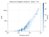
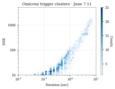
As a first step, I attempted to replicate the clustering approach from entry #66013 using only the Omicron trigger parameters (e.g., SNR, duration, central frequency). This approach did not yield clearly identifiable clusters. The issue is that parameters like SNR and duration seem to span continuous values without forming isolated regions in the Omicron parameter space. For example, Figure 1 shows a 2D histogram of glitch durations and SNRs recorded between June 7 and 11; although the line at SNR ~400 corresponding to the 25-minute glitches is faintly visible, it already does not constitute a distinct, separable group.
To better capture glitch morphology, I instead performed clustering directly on the whitened time series corresponding to Omicron glitch triggers with SNR > 100, yielding a total of 891 glitches between June 4 and 11 during DQ Studies mode. I applied hierarchical clustering using Pearson correlation as the distance metric (specifically, 1 - Pearson correlation). This method captures waveform shape and phase similarities while being insensitive to amplitude. The clustering procedure followed the method described here and in arXiv:1109.2378v1. The result is shown in Figure 2 as a dendrogram, where each leaf corresponds to a time series and the y-axis indicates dissimilarity. Branches connect waveforms that are more similar, and colors represent the identified clusters.
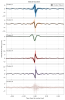
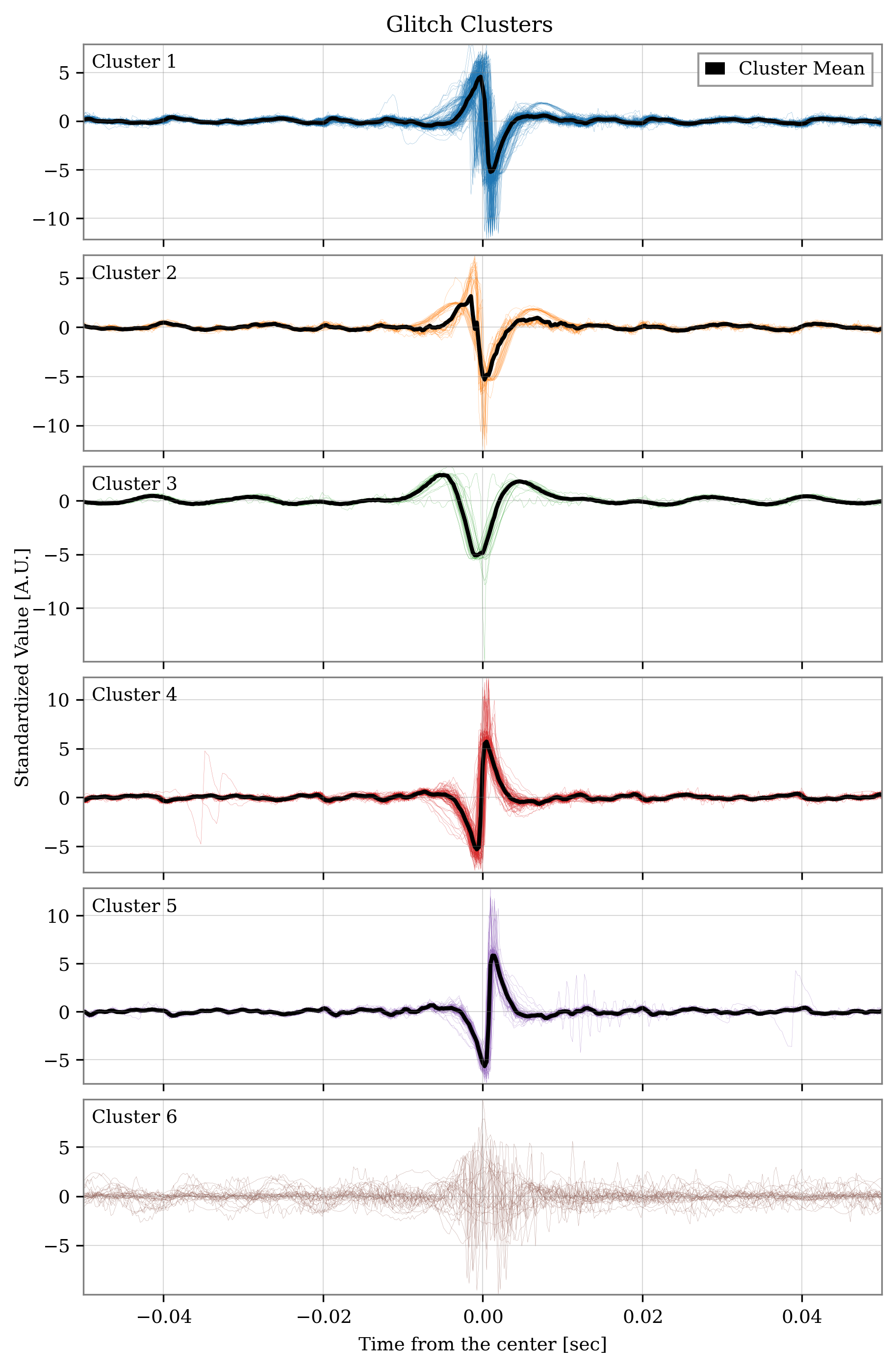
In Figure 3, I show the standardized time series for each cluster. The percentage of glitches across clusters is as follows: 41.44%, 8.95%, 4.86%, 23.74%, 15.37%, and 5.64% respectively. Clusters 1 and 2, and clusters 4 and 5, contain morphologically similar glitches that appear to differ by a phase of approximately Pi. Cluster 3 corresponds to the 25-minute glitches, while Cluster 6 contains a heterogeneous set of waveforms without a clear common structure. This suggests that the majority of glitches can be grouped into two dominant waveform types (each appearing with a phase shift), along with a third, distinct 25-minute glitch class, and a residual miscellaneous group.
I attach a CSV containing the GPS timestamps, center frequencies, and assigned cluster labels for all glitches.
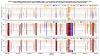
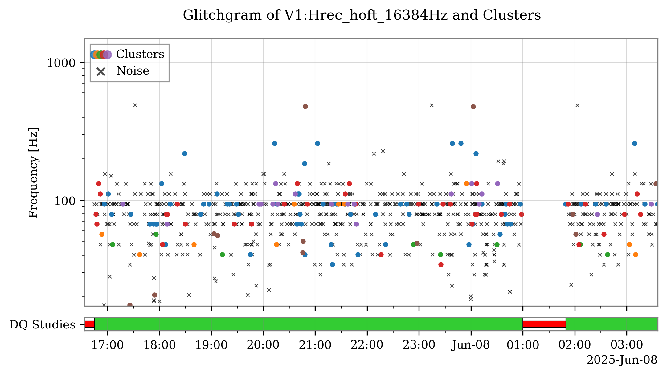
Figure 4 shows a glitchgram for the long segments in the DQ Studies mode between June 7 and 8, with each marker colored by its cluster assignment. As anticipated, the result is visually complex and does not reveal a clearly separable temporal or frequency structure among the classes.

Based on the shape of the glitches (specifically clusters 1+2 and 4+5), we can reasonably hypothesize they originate from step-like discontinuities in the strain: down-steps for clusters 1+2 and up-steps for clusters 4+5, respectively.
Interestingly, the directions of these jumps appear to be nearly balanced. While the previously reported percentages showed a majority in clusters 1 and 2, Michal has acutely noticed that some of the 25-minute glitches (Cluster 3) may have been misclassified into Cluster 1, which would bring the distribution closer to parity between clusters 1+2 and 4+5.
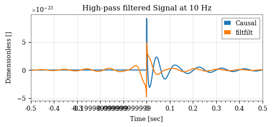
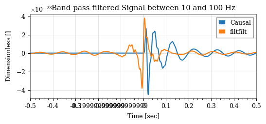
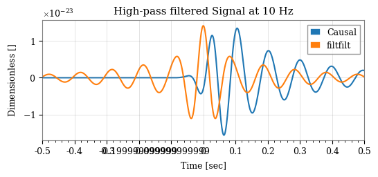
Regarding the waveform shapes, we can show analytically how a step function leads to the observed patterns in the plots, both in Michal's (with a causal filter) and mine (with a zero-phase filter). Here's a brief derivation:
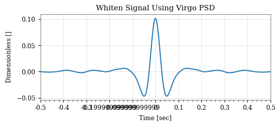
A unit step function u(t) (equal to 1 for t > 0, 0 otherwise) has a Laplace transform U(s) = L[u(t)]=1/s. The Virgo ASD behaves approximately like a high-pass filter, whose impulse response we denote g(t). Whitening the step function with the ASD, u(t)∗g(t), where L[g(t)] = 1/ASD(s), has a result similar to applying a high-pass filter. We consider, for simplicity, a first-order high-pass filter with transfer function G(s) = s/(s+ω0), where ω0 is the cut-off angular frequency. The transformed output is then: U(s)G(s) =1/(s+ω0), which corresponds to the time-domain function e^{−ω0t} u(t), that is, a decaying exponential starting at the step, the glitch. This matches the right-hand side of the waveforms in the plots for Cluster 4+5 (and is the opposite of Clusters 1+2).
When using a zero-phase (acausal) filter, such as the filtfilt method (which applies the filter forward and backward), the result becomes symmetric: combining e^{−ω0t} u(t) with its time-reversed counterpart −e^{ω0t} u(−t), forming a double exponential. The same reasoning applies in reverse for down-step inputs.
To explain the oscillatory features seen in Michal's plots, we can model the whitening process using a more realistic second-order filter, with transfer function: s^2 / (s^2 + 2ζω0 + ω0^2), whose response depends also on the damping parameter ζ . There are three main cases when applied to the step function: underdamped (ζ<1, e.g. Butterworth filter with ζ= 1/sqrt(2)), that characterizes an oscillatory response, critically damped (ζ=1) and overdamped (ζ>1), both of which present no oscillations and an approximately exponential decay. For example, for a Butterworth filter, setting ω0 = 1 to simplify the expressions, the filtered step function is: s / (s^2 + sqrt(2) +1) = (s + 1/sqrt(2)) / ((s+1/sqrt(2))^2 +1/2 ) - (1/sqrt(2)) / ((s+1/sqrt(2))^2 +1/2 ), whose inverce Laplace transform can be read from this list: e^{-t/sqrt(2)} [cos(t/sqrt(2)) - sin(t/sqrt(2))] u(t).
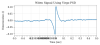
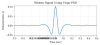
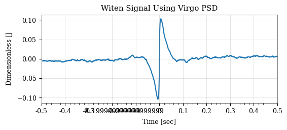
Moving to simulated data, I’ve attached:
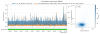
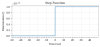
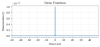
Figure 1: Plot of a step function,
Figure 2: Its whitened version using the Virgo PSD,
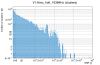
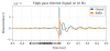
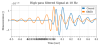
Figures 3 and 4: The filtered function by a high-pass (cut-off = 10 Hz) and band-pass filtering (10 -100 Hz).
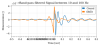
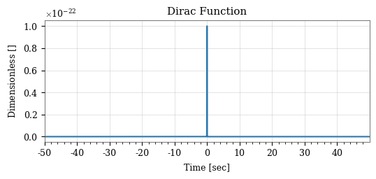
For comparison, I also add the same plots for a filtered Dirac Delta function ( ~ 25 minute glitches): Figures 5-8.
In conclusion, the new class of mid-frequency glitches appears to be generated by step discontinuities in the strain. It is therefore quite appropriate to refer to them as "step glitches".
PS: I am no longer able to use codecogs to write equations in the logbook!! :-(
I have run a similar analysis to entry #66972 by modelling each glitch waveform with a Virgo dedicated version of DeepExtractor (https://arxiv.org/abs/2501.18423), which allows to extract excess power from a whitened timeseries. I used as glitch triggers a threshold over the channel V1:DQ_BRMSMonHrec_BRMS_HREC_HOFT_FREQ_BAND_85_95_Hrec_hoft_16384Hz as proposed in entry #66923. I ran the algorithm on a long stretch of data when the interferometer was locked on the 11th of June. Clustering has been done with DBSCAN using 1-pearson correlation as a distance metric. The results are very similar to the previous entry. I have used very conservative DBSCAN parameters to reduce the number of "outliers" in each class.
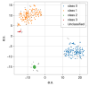
Figure 1 shows a projection in 2D of the dataset using t-SNE algorithm, just for visual purposes.
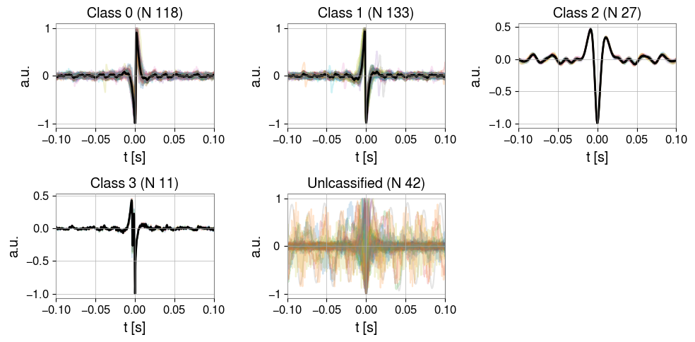
Figure 2 shows the median class waveforms. Each waveform has been rescaled to have compatible amplitudes. Classes 0 and 1 correspond to the up-step and down-step glitches, class 2 is the 25-minute glitch, while class 3 seems to be a subset of the up-step class. The number of up and down steps is quite similar. Note that due to the DBSCAN settings, some step-glitches ended up being unclassified.
I will try and run the algorithm on longer stretches of data to gain more GPS times.

This is interesting. Class 3 of glitches may be related to B1 photodiode audio channel saturation, either for other reasons, or caused by the tail of the loudest "step" glitches. It would be nice to check if the class 3 glitches correspond to times where the channels SDB2_B1_PD1/PD2_Audio_saturation goes from 0 to 1.
I have taken the GPS times from class 3 glitches, and this seems to be the case: every time a glitch in this class occurs, the photodiode saturates.
Figure 1 shows the channel SDB2_B1_PD1_Audio_saturation observed at each GPS time identified by the class 3 glitches. The channel goes from 0 to 1 every time.