I complement Didier's analysis with a few plots.

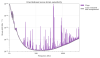
In Fig. 1 I have created a spline curve (grey line) to approximate the Virgo sensitivity curve, without all the spectral lines. Notice that this curve has a general tendency to underestimate the strain ASD (or overestimate the sensitivity: don't trust the reported range!).

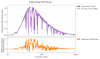
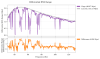
From the above curves, I have plotted in Fig. 2 and 3 the Differential BNS Range. This quantity (reported also on VIM in the CAL Summary page) is the square root of the integrand in the BNS range equation multiplied by the frequency, and then integrated over d(ln f) = df/f, as suitable to be shown on a logarithmic x-axis. The orange curve at the bottom is the difference in the differential ranges of the actual Virgo data and their spline approximation. Notice that this orange curve is almost everywhere above zero, due to the aforementioned bias in the model. Evident are the frequency regions reported by Didier: the structure around the 50 Hz, that around the 63 Hz line, and 74.4 Hz line. Additionally, it is visible how a considerable part of the sensitivity is obtained between 30 and 100 Hz. The line at 41 Hz has also a significant contribution.

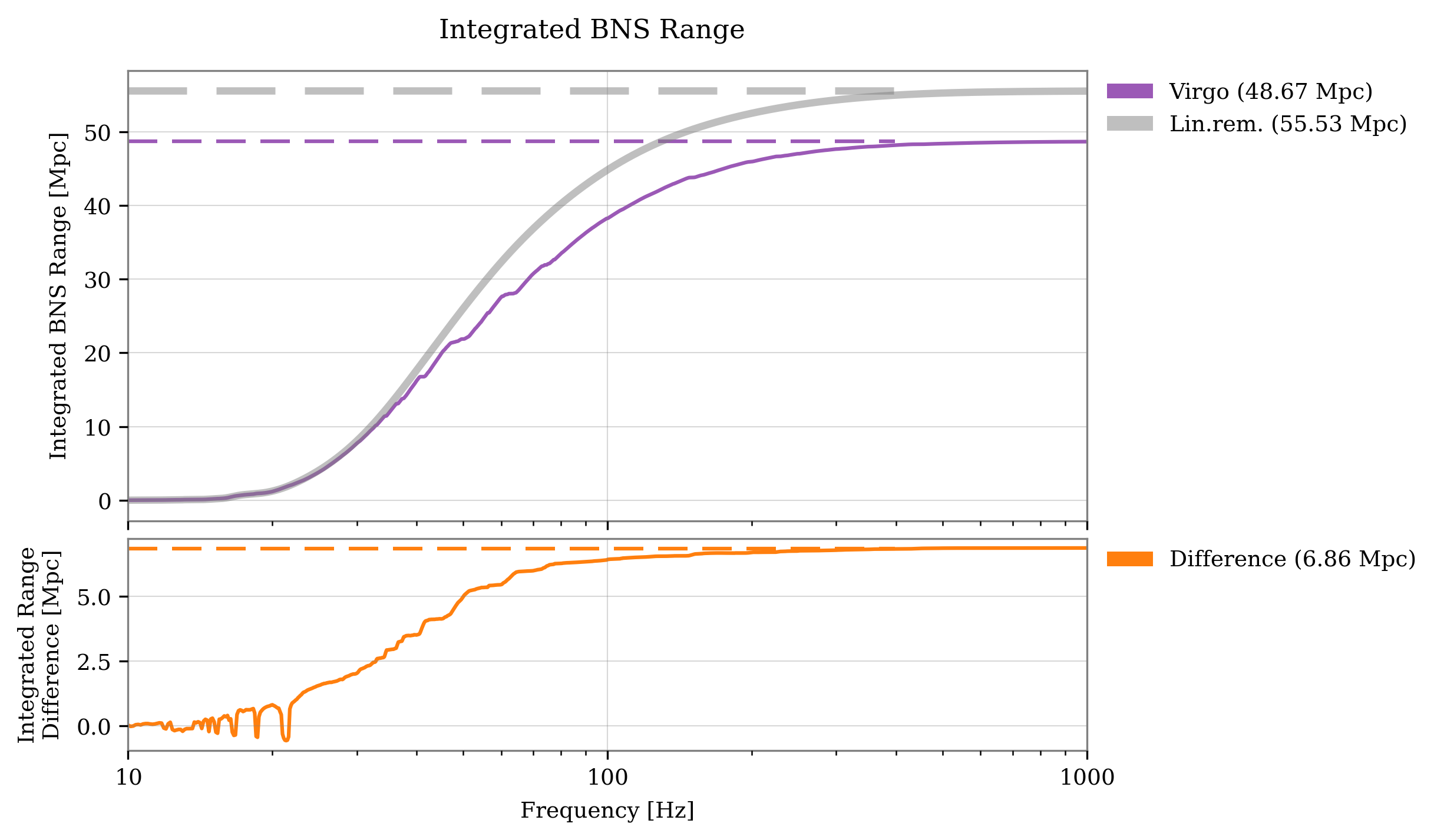
Figure 4 shows the integrated range for the actual and approximated sensitivities, and their difference. Here you can see that a range of about 40 Mpc is obtained just in the region below 100 Hz. The steps in the orange curve represent again where most of the range is lost.