The etalon fringes as the loop is turned and sweep through several fringes of the etalon effect in the input mirrors is modulating the BNS range.

Figure 1. Corresponds to the case of a high BNS range.

Figure 2. Corresponds to the case of a low BNS range.

The frequency noise projection is not playing a significant role. The DARM gain is different by 3% between the two cases so it is also not a dominant contribution. What varies to explain the sensitivity curve is the level of mystery noise in mW/rtHz units, they are different by ~20%, which explains most of the BNS range changes that are of 15% between the two cases. The BNS range varies less, because in the sensitivity curve there are also other noises than just the mystery noise, and these do not vary.

/users/mwas/detchar/toySensitivity_20260116/toySensitivity.m

I'm trying, as usual, to do a personal decomposition of the noise curve. I start putting some known components, which should be not far from the ones used in Michal's budget. I also put a manual copy of many large structures visible in the noise above the floor. Then I add a few parametric curves and I run an automatic search of the best parameters allowing a good fit of the sensitivity with those curves.

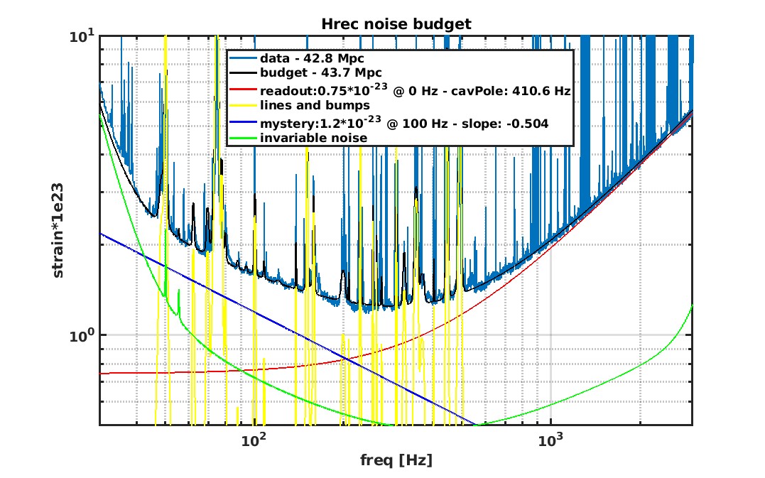
I did an attempt on the best data found yesterday (gps 1452475518, dur 800 s, 37.5 Mpc, DCP 430 Hz). The additional curves are:

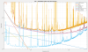
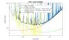
- a constant in DARM, multiplied by a zero at DCP, to match the calibrated shape of Hrec - this is indicated as 'readout noise'

- a curve with a constant slope in DARM, multiplied by a zero at DCP - this is indicated as 'mystery noise'.

The slope is used as a parameter of the search together with the amplitude of the two curves.

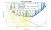
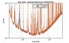
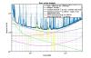
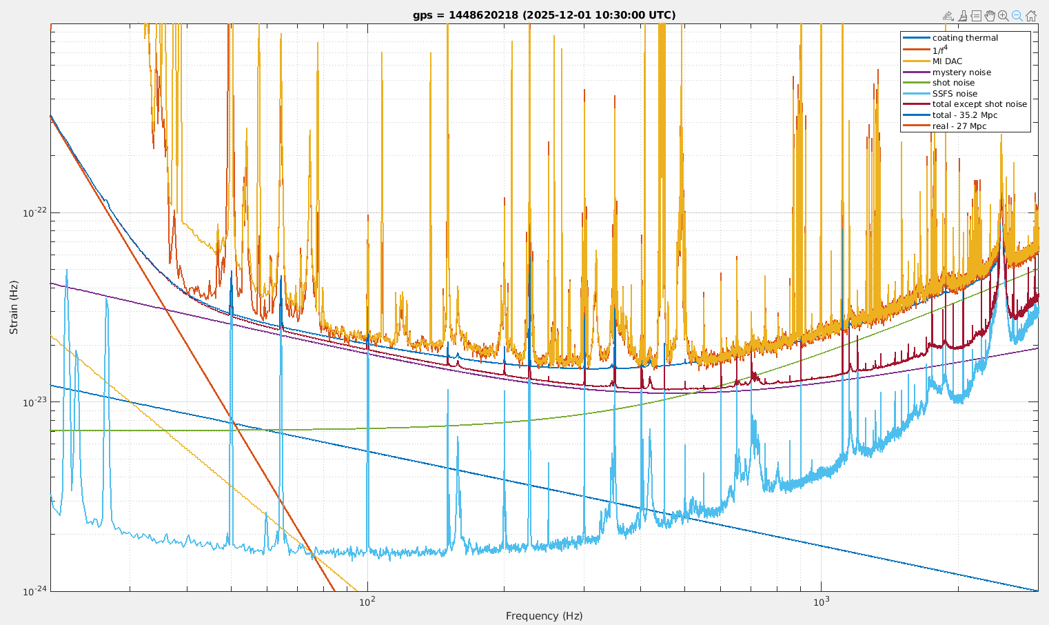
The result, shown in fig 1, gives an astimation of the slope -0.679, very close to first estimation of 2/3. Unfortunately the fit clearly overestimates the noise around 90 Hz and 45 Hz, saying that the slope could be lower. In that case, the quality of the fit become worse at higher frequency, but there is no reason to rely too much on the method and conclude that no constant slope can reproduce the mistery noise.

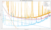
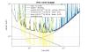
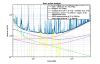
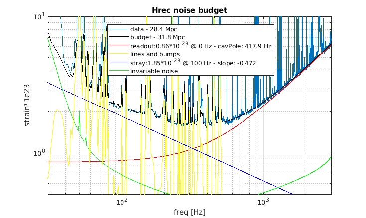
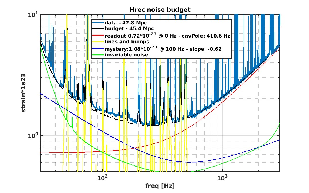
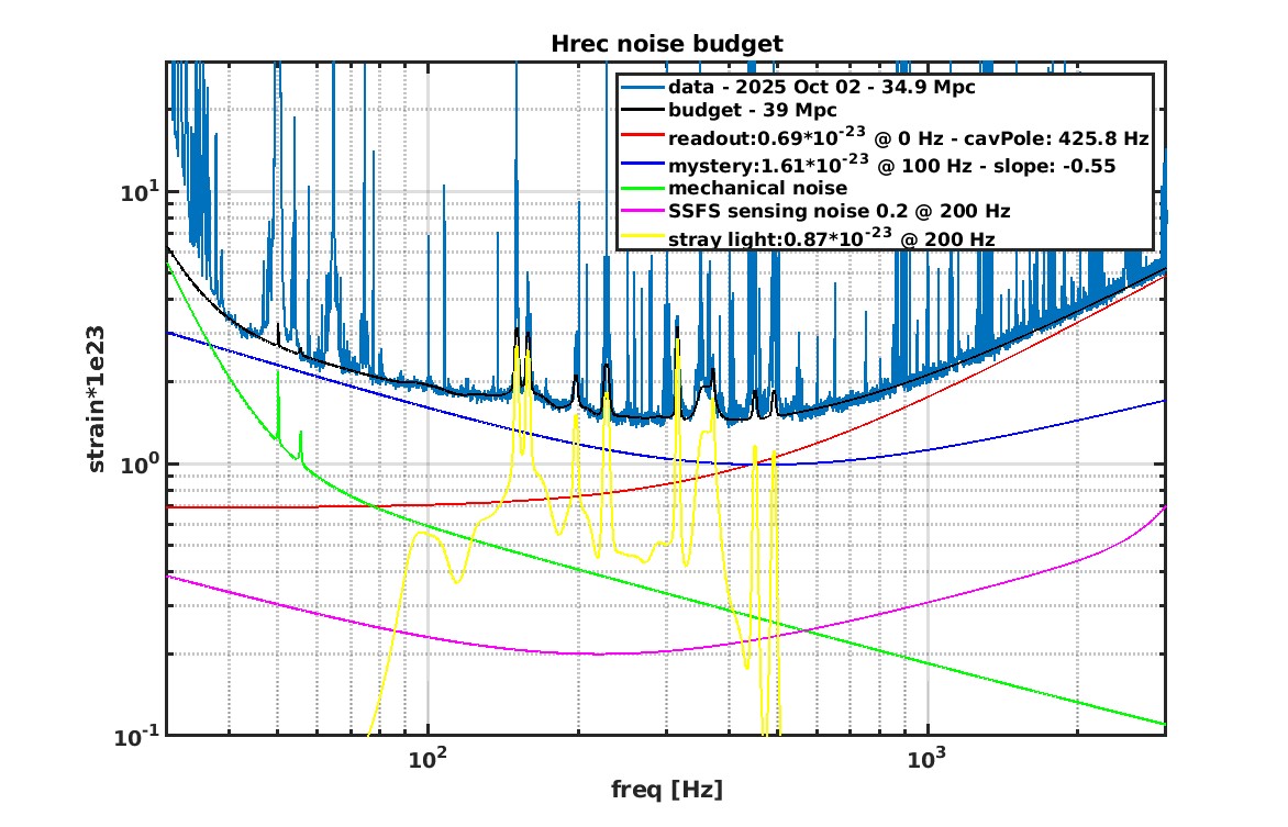
Anyway, I tryed a different assumption: a constant slope in Hrec. I know that this is a strange assumption, because an optical noise should have a simple shape in DARM and the zero due to DARM response should be applied in any case. My assumption is done for its simplicity and correspond to the case of a noise with constant slope at low frequency and some cut-off in the frequency region of the DCP.

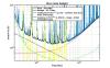
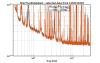
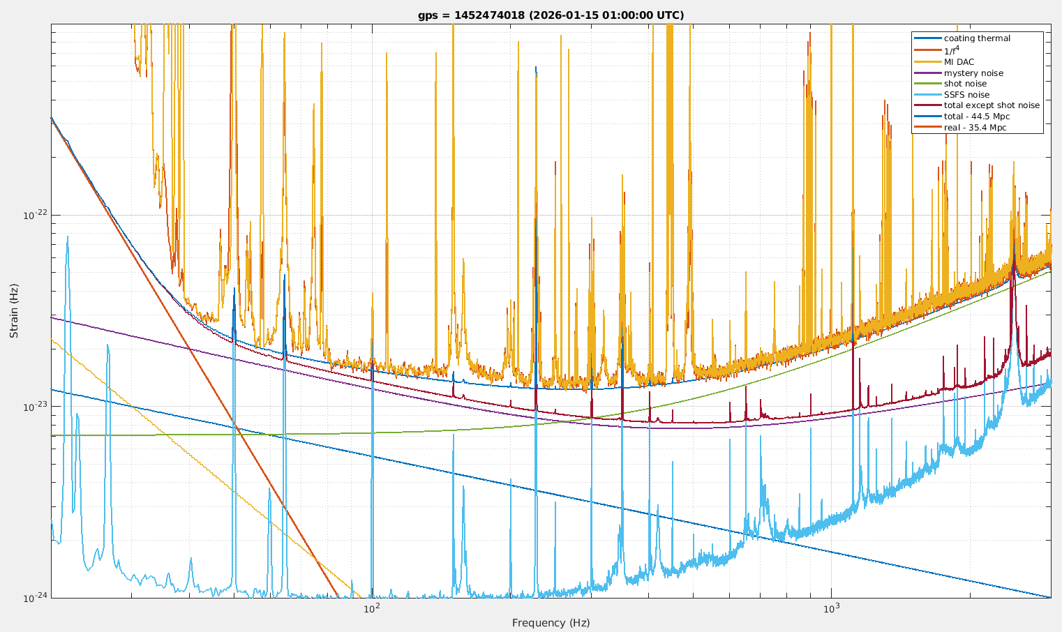
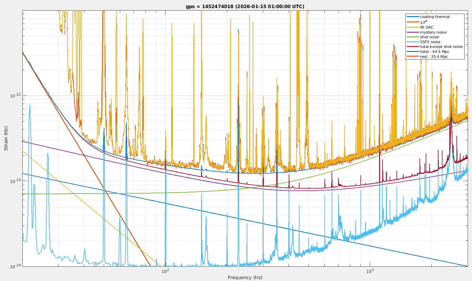
The result is shown in fig 2: it gives an estimation of slope -0.425 and it is very satisfying everywhere. It is so much satisfying also because I built the bumps and lines starting from this fit, so I arbitrarily covered some discrepancies, but I did not make any relevant change of the floor. The parameter search has been done keeping in the game also a mystery noise component with fixed slope 2/3: the result for its best amplitude has been 0. In the plot, the new curve is called 'stray' just to distinguish it from 'mystery'; the name is not a hint concerning its possible nature.

The second fit forces the readout noise to be a bit larger that in the first fit. If there is a precise indipendent estimation of the readout noise, which is lower than the sensitivity curve, the second model of excess noise cannot fill the gap and should be discarded. But there is also the possibility that the gap is due to another mystery noise, coming from a different source.

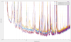
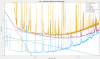
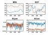
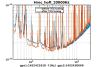
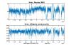
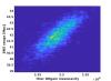
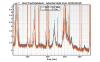
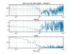
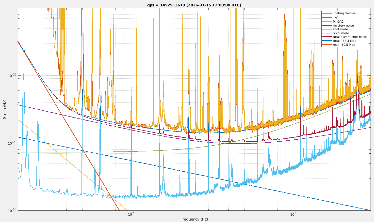
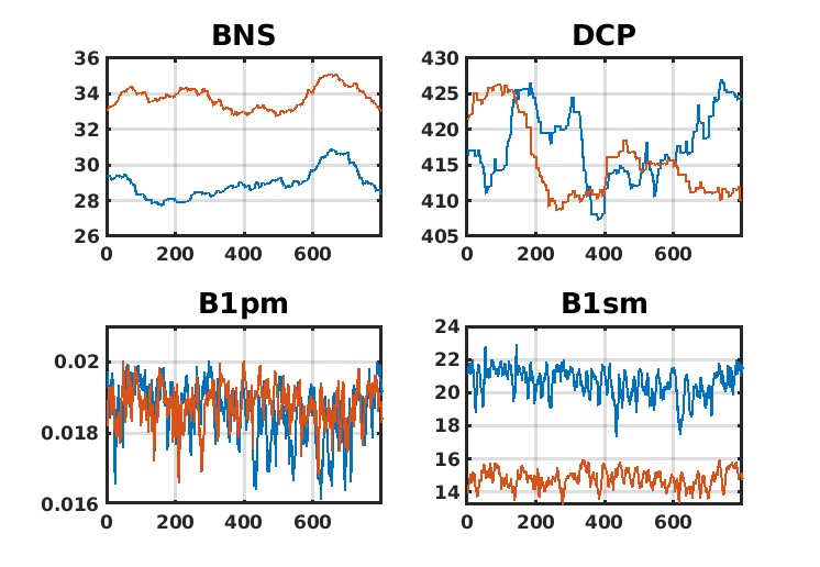
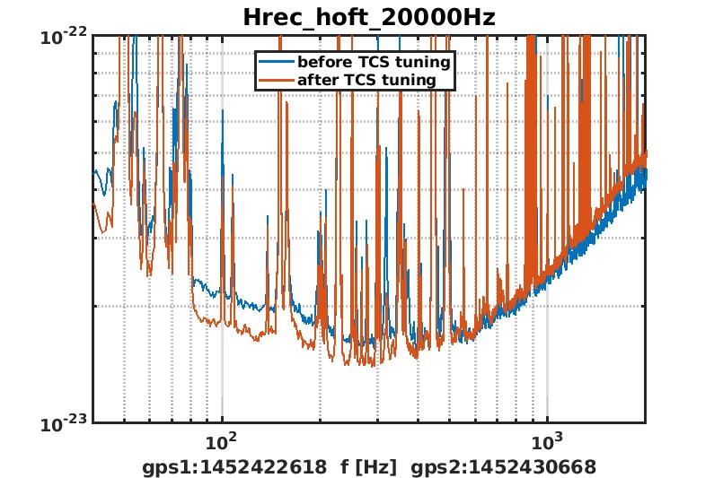
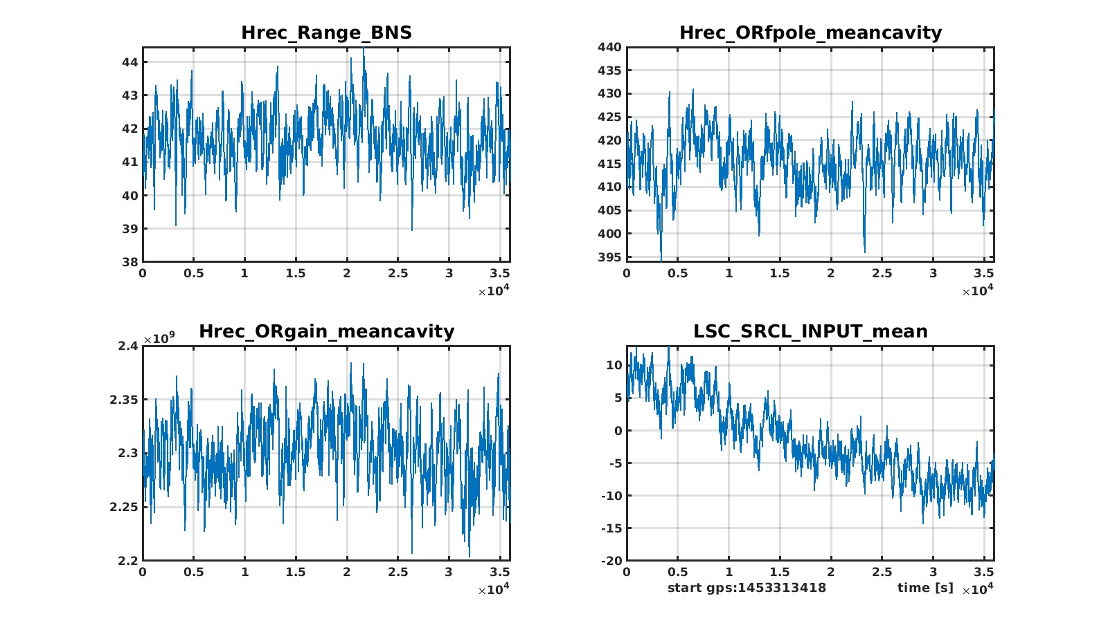
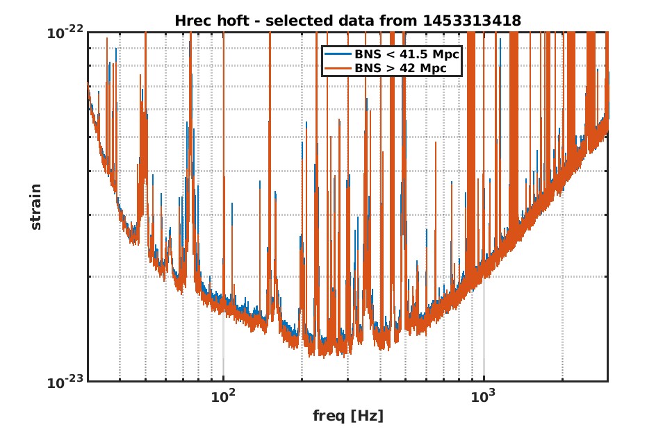
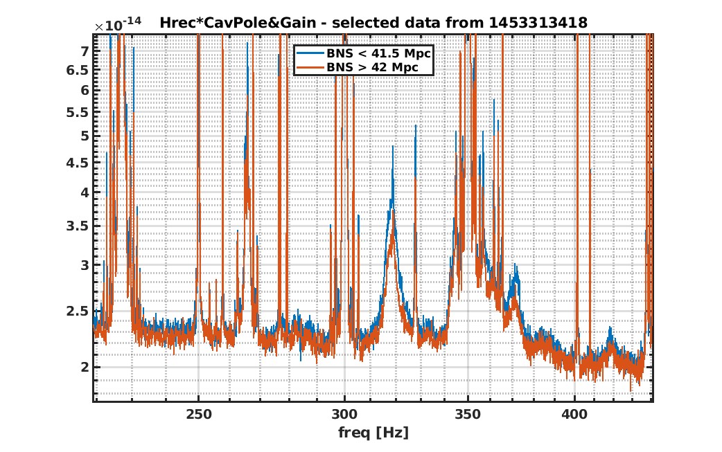
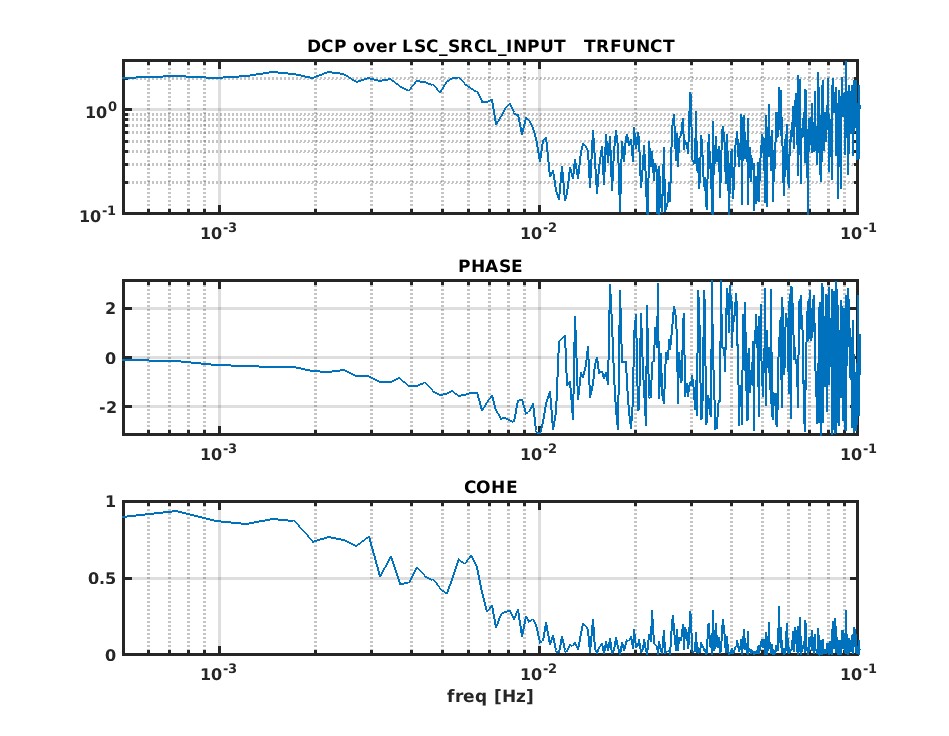
I tried to use the low-passed model of mystery noise also for different data. In particular, I was very curious about the very bad data collected before the TCS adjustment which removed the big problem on B1s. In fig 3, blue curves, some characteristic figures of merit of that working point are shown, compared to the ones obtained two hours later by a translation of WI DAS. The differences are a much darker B1s, with no change of B1p, and a higher range. The increase of the range looks like a big reduction of mystery noise (fig 4). The two curves are different also regarding the amplitude of some well kown structures normally associate to stray light. This is not surprising: always happened that more light coming out from the dark port creates problems of stray light and problems of sensitivity.

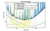
The application of the automatic fit to the bad data (before TCS tuning) gives an acceptable result (fig 5) and an estimation of excess (mystery?) noise 50 % larger than the one obtained for the very good data analysed in the first plots.

I will draw some conclusions from this analysis:

- The sensitivity we can observe with SR aligned is largely dependent on the working point tuning. The effect on the sensitivity of the diafragm installed on SR can be somehow covered by other changes and any attempt to make pre-post comparisons faces that difficulty.

- We should not exclude the presence of different sources of noise affecting the sensitivity in this complicate state of the ITF. If we want to evaluate the amplitude, the shape and the variability of the specific noise we use to call 'mystery' noise, it should be better to minimize the noises that can have more normal explanation, like the stray light. As the mystery noise, the stray light depends on HOM content in the dark fringe and can put some bias in our attempt to have a precise correlation between HOM and some 1/sqrt(Hz) shaped noise of different origin.

The data collected during the weekend in LN3 ALIGNED were quite good in terms of BNS range and not bad in terms of DCP stability (fig 1). Selecting several segments in good and homogeneus conditions, I computed a high resolution higly averaged sensitivity curve and I tried to extract a fit of the noise components. Using the automatic fit which tries to superpose the best curve to the noise floor, the curve in fig 2 came out, giving again an estimation of mystery noise slope -0.5. Unfortunately, using high resolution data shows quite clearly that the method overestimates the noise floor.

A similar search, done manually with the constraint of staying below the curve everywhere, gave a different result, both regarding the amplitude and the slope of the mystery noise (fig 3). In this case, a higher slope needs to be used (my best choice has been -0.62). It is also worth to notice that a polynomial component can explain only partially the noise floor: the excess noise contains a relevant part of 'irregular' noise, which needs to be explained too. The presence of this additional componet could add uncertainty in the quantification of an indipendent polynomial component.

Concerning the non-stationarity of the noise, I can only remark that BNS_Range fluctuations always follow the modulation of DARM optical gain at low frequency. Looking for instance at the very good 10 hours data collected on January 24 evening-night (fig 1), one can find a perfect linear correlation between Hrec_Range_BNS and HREC_ORgain_meancavity (fig 2).

I did two different selection of segments in this period:

40.2<BNS<41.45 - minimal duration 150 s - total duration 4241 s

42.1<BNS<43.5 - minimal duration 150 s - total duration 4212 s

Hrec spectrum (fig 3) changes uniformely everywhere in the critical region.

Assuming that Hrec_hoft is obtained using the information about DARM response stored in the two HREC meancavity GAIN & POLE channels, I reconstructed segment by segment an hypotetic open loop DARM spectrum from Hrec_hoft spectrum. The averaged spectrum (fig 4) shows a much lower variation of noise in the floor. Zooming around some typical structure of the noise (fig 5), one can see that the variations are more evident in the lines and bump, instead of the floor. I don't know what does it means. I just add that the control signal more involved in this kind of modulation is LSC_SRCL_INPUT, the one created to keep the Arm optical spring as low and stable as possible. The impact of that signal on the ITF working condition is quite evident looking at its transfer function and coherence with the Double Cavity Pole of the arms (fig 6). We also know that the disturbance on the DCP stability worsen when the measurement of the optical spring is worse. Fluctuations of the optical spring possibly linked to SRCL working point fluctuations could induce variations of arm mechanical response by a few % even at 70 Hz, producing some bias in the estimation of DARM optical response parameters.

I tried to improve the automatic decomposition of Hrec, in order to adapt it to SR ALIGNED data. The aim is to have a not too arbitrary method of comparing the amplitude of the mystery components at different gps.

I started from October 2nd data, before the diaphragm installation. In order to correct evident discrepancies between data and fit, I built a specific 'irregular' component, reported in fig 1 as 'stray light'. After some iteration, in which the mystery noise slope has been assumed as a parameter of the fit together with the amplitude of mystery noise, readout noise and stray light, a slope of -0.55 has been chosen. In fig 1 also the frequency noise component is explicitly shown; this is not included in the automatic search of parameters, but it is a variable component. The variability depends from the different CMRF, monitored by the channel LSC_DARM_SSFS_LF_COUPLING. There is an initial assumption of noise level for a given CMRF, then the level is rescaled according to the actual CMRF. The initial assumption needs to be checked.

The automatic fit has been applied to recent good data, keeping the same slope of the mystery noise and the same shape of the stray light component. The accordance to the data is not too bad, as shown in fig 2. The new mystery noise level is 69 % of the old level. The new stray light level is 56 % of the old level. There is also a relevant change of frequency noise; the uncertainty of its estimation could affect a bit the estimation of the other parameters, but not too much.