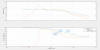
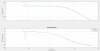
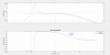
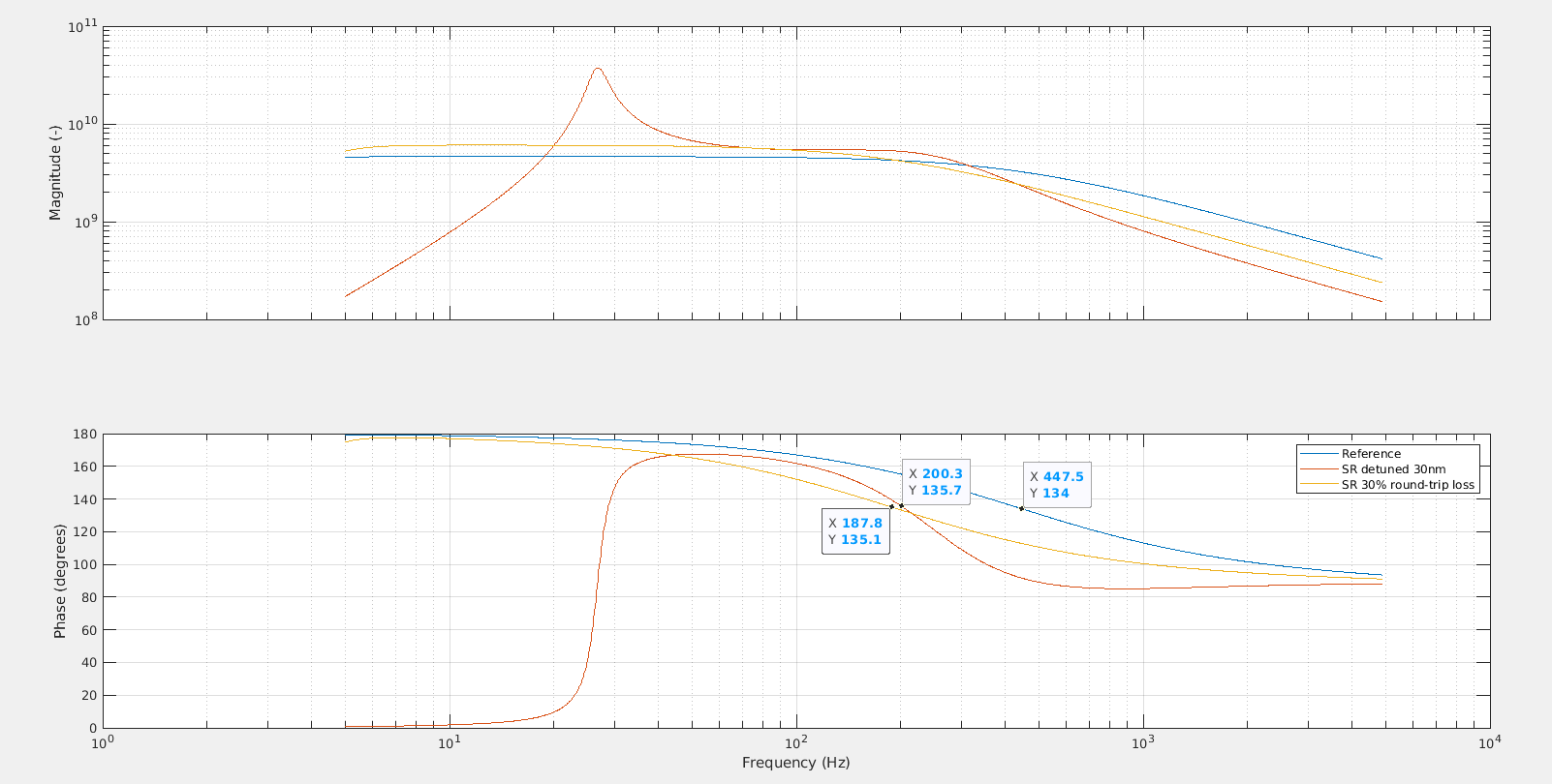
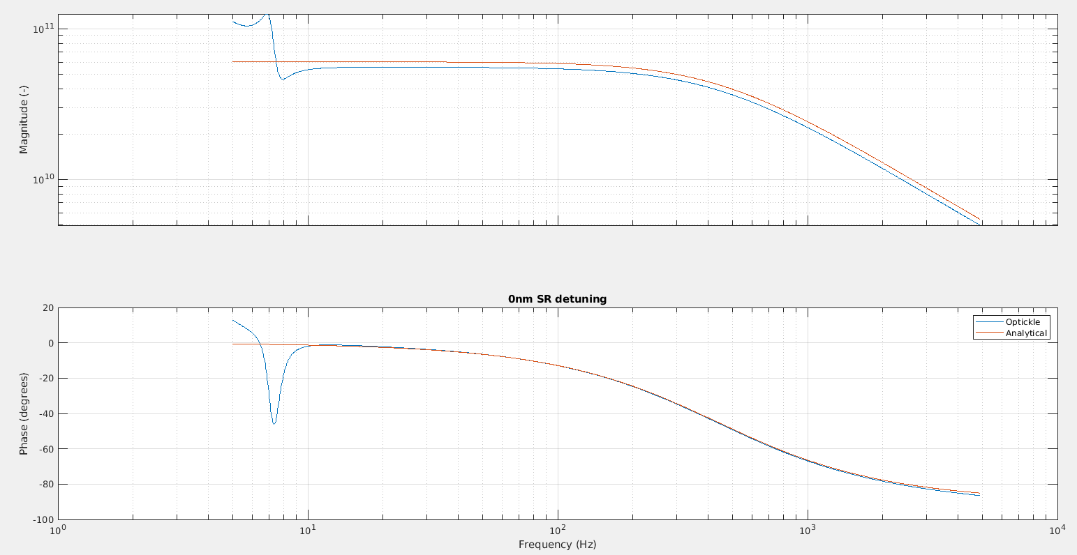
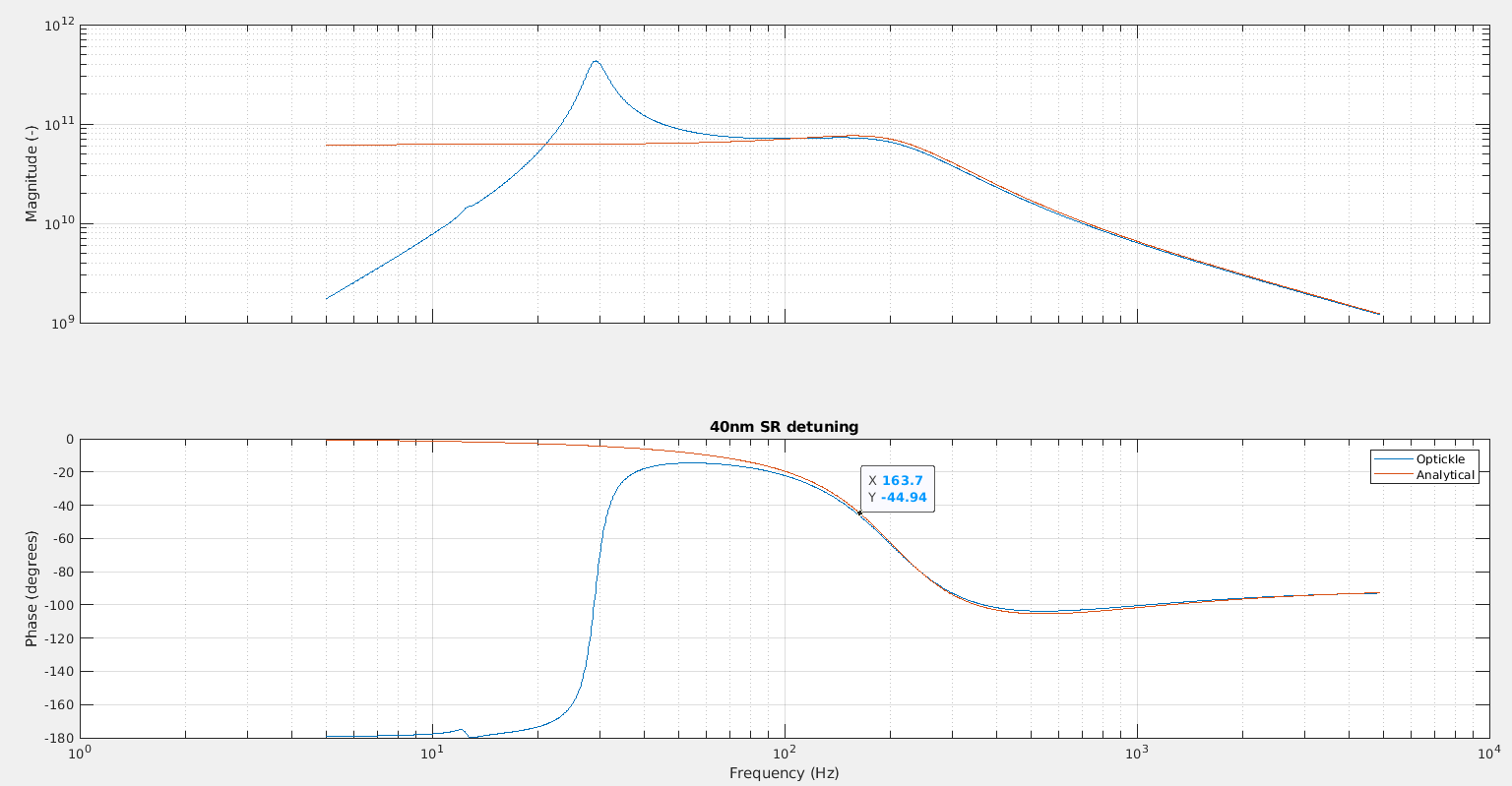
Figure 1, 2 and 3 show three cases of SR detuning (0nm, 10nm and 40nm). With a numerical computation done with Optickle that includes radiation effects, and an analytical computation (without radiation pressure effects). The analytical computation amplitude have been scaled by a factor 1e10, to approximately match the simulation.

In the analytical computation the optical spring is not present as there is no feedback or radiation pressure in the analytical computation. Above 100Hz the analytical computation matches well the phase evolution of the simulation, even for the 40nm case that has the optical spring at 30Hz. So the phase evolution at high frequency is not an effect of the optical spring itself. It is an effect of the SR detuning (which affects both the double cavity pole frequency and the optical spring frequency).

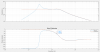
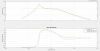
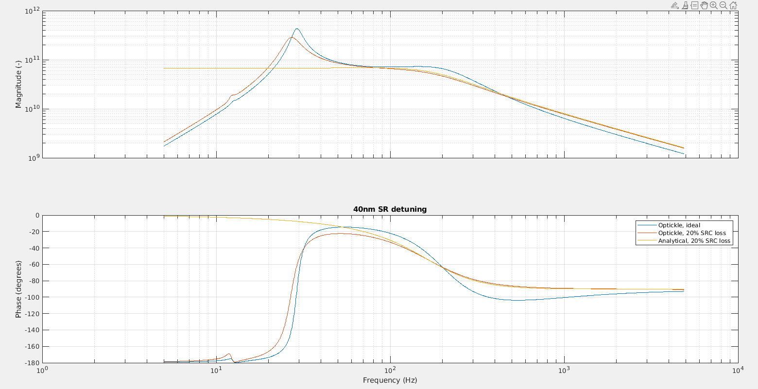
Figure 4 shows the case of SR detuned with and without large (20%) losses in the SRC. The analytical computation also gives the same phase evolution above 100Hz as the optickle simulation for the large losses.

The analytical compuation is based on the 3 mirror coupled cavity derivation in Andre Thuring PhD thesis from 2009, section 2.2.1, especially equation (2.52).

In principle from the shape of the optical transfer function phase above 100Hz we should be able to extract both the detuning of SR in nm, and the SRC losses. But including the information of the optical spring into the fit, may make it more reliable, assuming that the effective SR detuning is the same for the optical response and for the optical spring.

The matlab/octave script to make the analytical computation is attached. I expect that the expressions can be further simplified (by neglecting the length of the SR cavity completely, and evaluating analytically the final term).

One can fit a second order zero-pole filter response to that analytical optical transfer function. In general it gives results like the one below (example for 40nm detuning of SR and 10% SRC losses). In this example the fit has simple zero 325Hz, and a resonant pole at 189Hz. The frequency of the zero is affected only by losses, without losses it would move to the design value of ~440Hz. The frequency of the resonant pole is mostly due to the detuning of SR, but is also changed by losses. When the detuning gets smaller the pole moves closer in frequency to the zero. With no detuning the simple zero and resonant pole overlap giving the simple pole we expect. So by fitting a second order filter, we could try to measure directly the SR losses, from the measured zero frequency, and the resonant pole frequency tells us that the SR position is detuned.

zpkTF =
 
  9.7291e-05 (s+4.549e07) (s+2043)
  --------------------------------
      (s^2 + 1455s + 1.407e06)
 
Continuous-time zero/pole/gain model.

zf =
       325.12
     7.24e+06
zq =
     0
     0
pf =
       188.76
pq =
      0.81507