Following the measurement last march that end benches scattered light couples through radiation pressure. I have implemented an Optickle simulation of the SNEB, SWEB, SDB1 and SIB1 scattered light coupling transfer function, by adding 1ppm mirrors at their position into the model. This follows the approach implemented by Gabriele Vajent back in 2012, VIR-0254A-12.
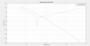
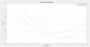
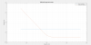
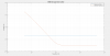
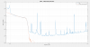
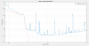
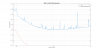
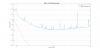
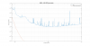
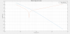
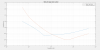
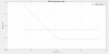
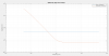
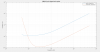
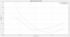
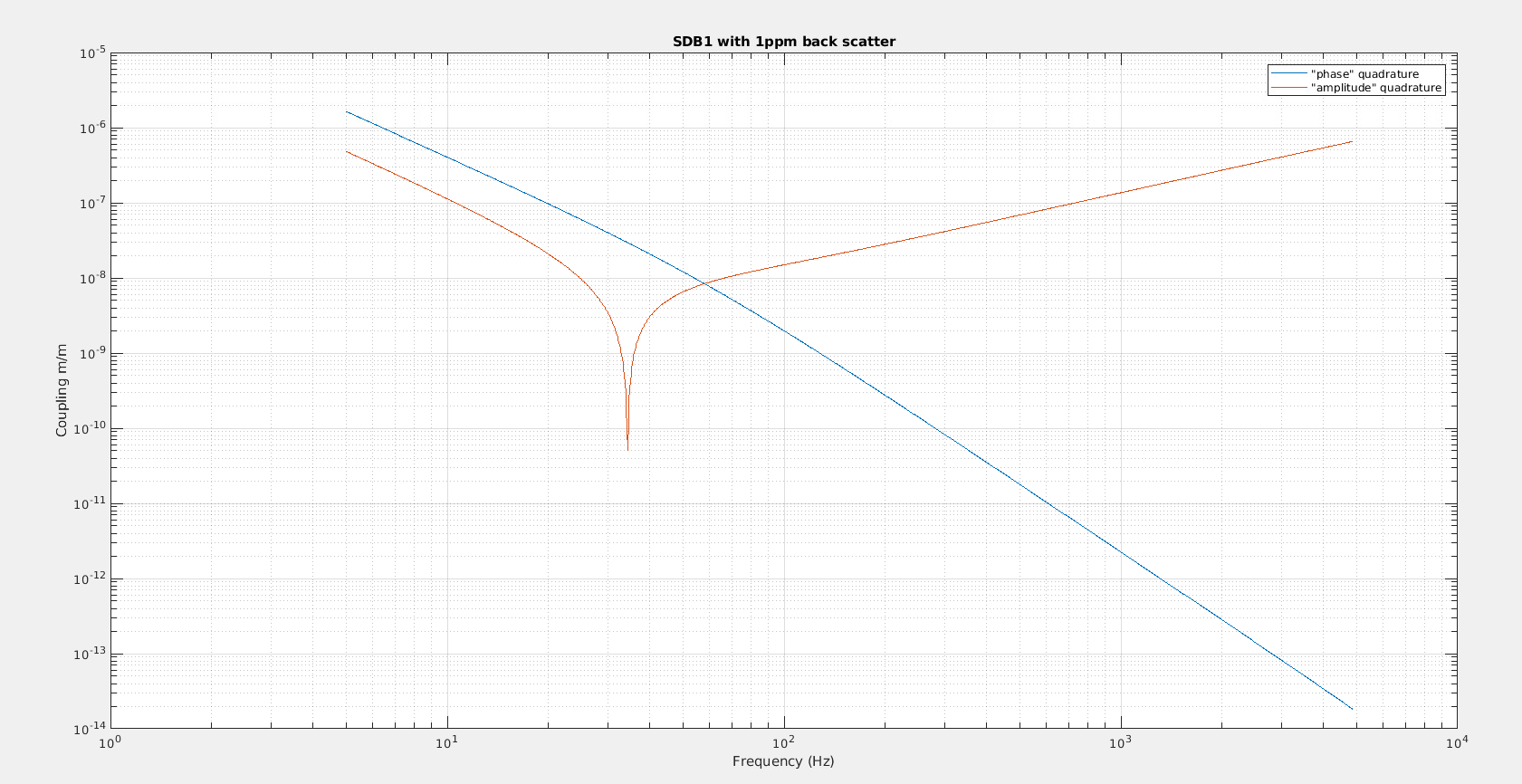
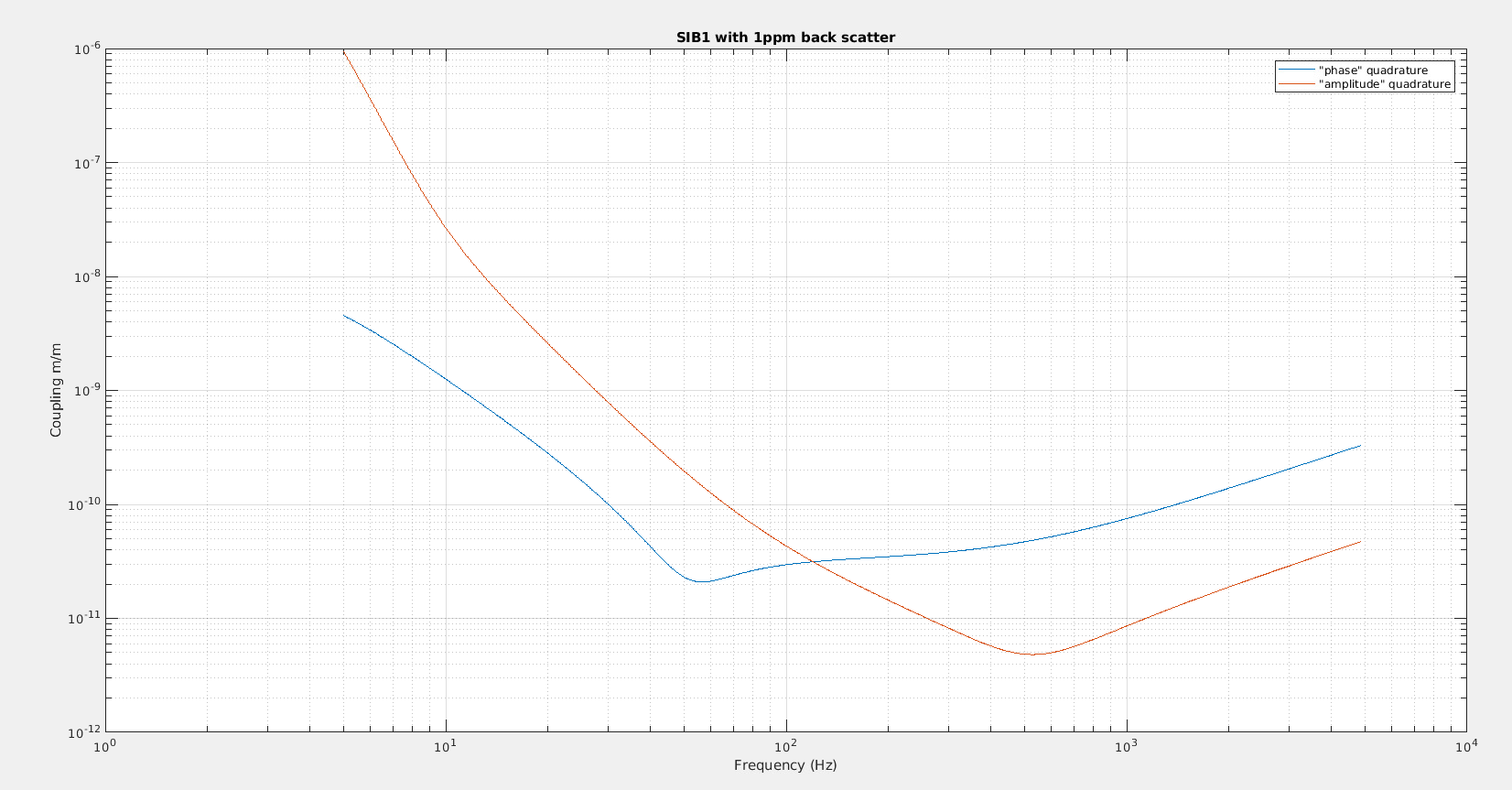
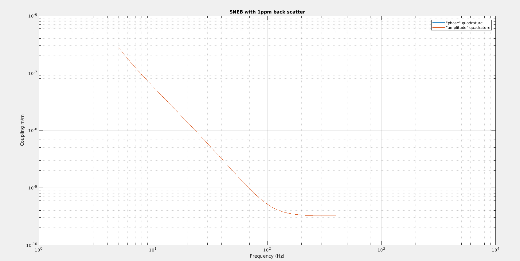
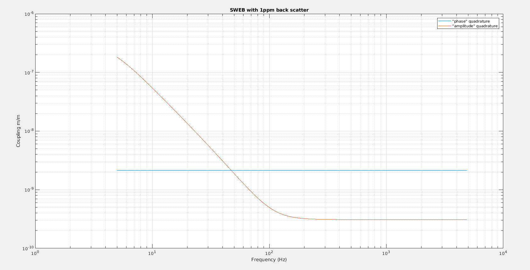
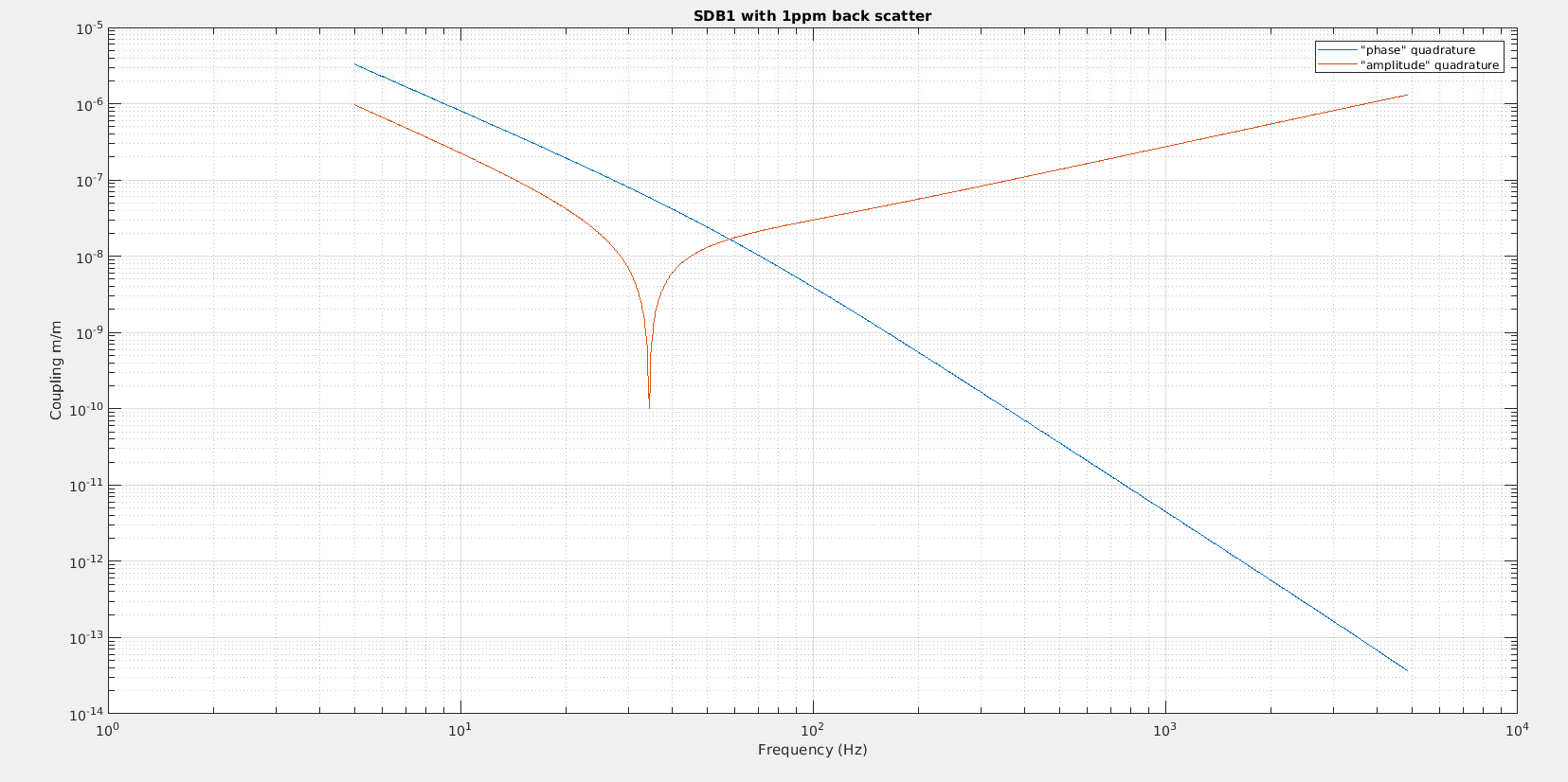
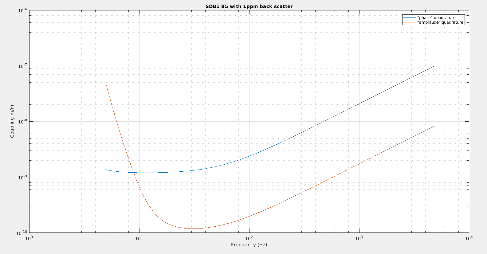
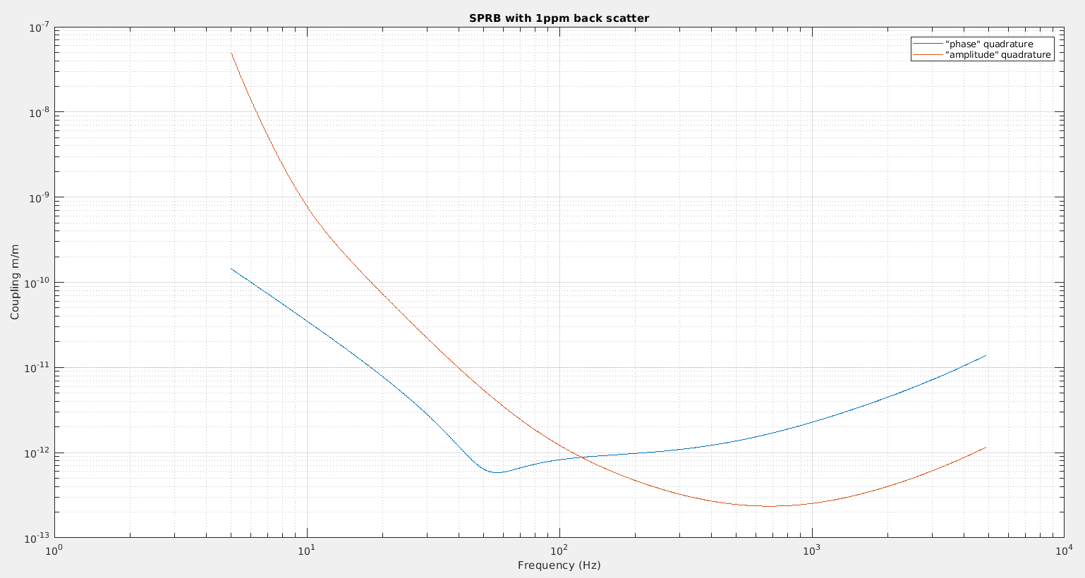
The main function for this can be found on the noise budget SVN. Figure 1-4 shows the result in terms of transfer function between bench motion in meters and DARM equivalent noise in meters, assuming the bench backscatter 1ppm of power that perfectly recombines with the ITF beam. The result for SDB1 and SIB1 are of the same orders of magnitude as the Gabriele's result (that were for a different configuration of 125W laser with SR in a detuned position for optimal BNS range). There are two quadratures for the coupling, depending on the microscopic position of the scatterer (the two position are separated by pi/8*wavelength), and I have check that all other position are an interpolation of these two quadratures, as Gabriele also shows in his presentation. The names in the legends are somewhat arbitrary they actually correspond to 0 and pi/8*wavelength microscopic position in Optickle.
Dividing by the arm length (3000m) this transfer function become couplings between bench position and h(t), this couplings transfer functions are available on the SVN. However, the bench scattered light coupling is not linear due to fringe wrapping. Hence the bench motion needs to convert to scattered light phase before using the linear transfer functions.
noise_phase_quadrature = tf_phase_quadrature/3000 * 1.064e-6 / (4*pi) * ASD( sin (4*pi/1.064e-6 *x_bench)))
noise_amplitude_quadrature = tf_amplitude_quadrature/3000 * 1.064e-6 / (4*pi) * ASD( cos (4*pi/1.064e-6 *x_bench)))
Whether the sin or the cos of the bench position needs to be used for each quadrature in the equations above may not be correct, but it doesn't matter in this application as the bench position sweeps many fringes so the spectrum of the sin and the cos are the same. I then assume that the two coupling paths add in quadrature. This is not correct as the two may interfere, but at most frequencies one of the coupling paths dominates over the other. So only where two couplings cross the projection may be too small by a factor sqrt(2) (if the interference is constructive), or by overestimated (if the interference is destructive).
This can then be applied to project the noise of suspended benches and measure their back-scatter in terms of PPMs, as the transfer function scales as the square root of the back scattered power.
For SDB1 and SDB2 there are measurements available from March 2019
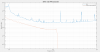
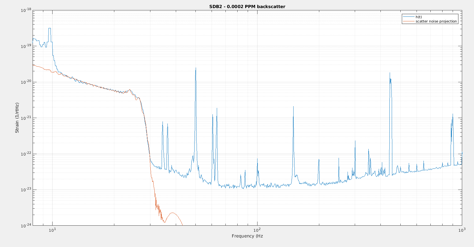
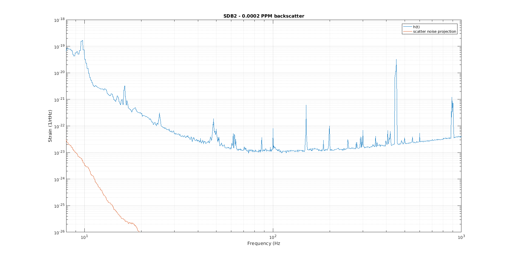
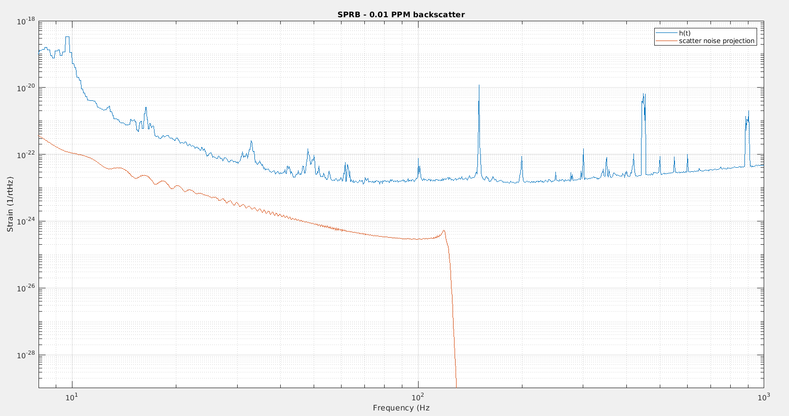
Figure 5 shows that for SDB2 the back scatter projection matches perfectly the measured coupling in h(t). And it corresponds to 0.0002 PPM of back scattered power. However for the B1 path there is a Faraday isolator on SDB1 that filters out light back scattered by SDB2. Assuming a 37dB rejection, this correspond to 1PPM of light back scattered by the bench itself.
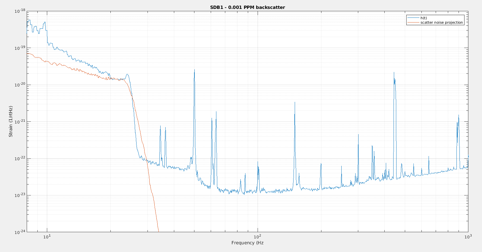
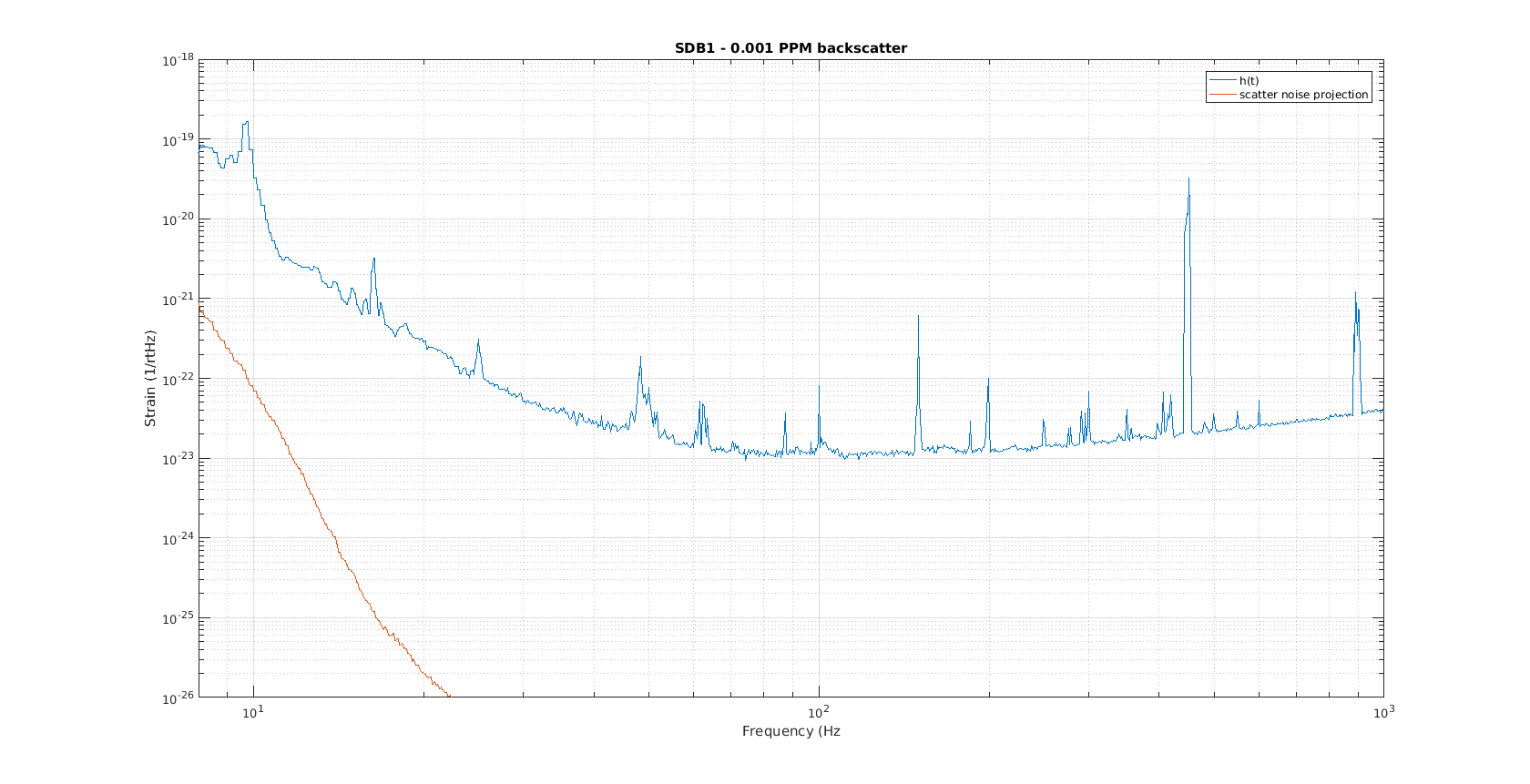
Figure 6 shows that for SDB1 the projection does not work well. It may be that the back scattered light doesn't couple through DARM, but through a different loop (for example MICH). Or that the dominating back scatter is not on the B1 path, but on the B5 path.
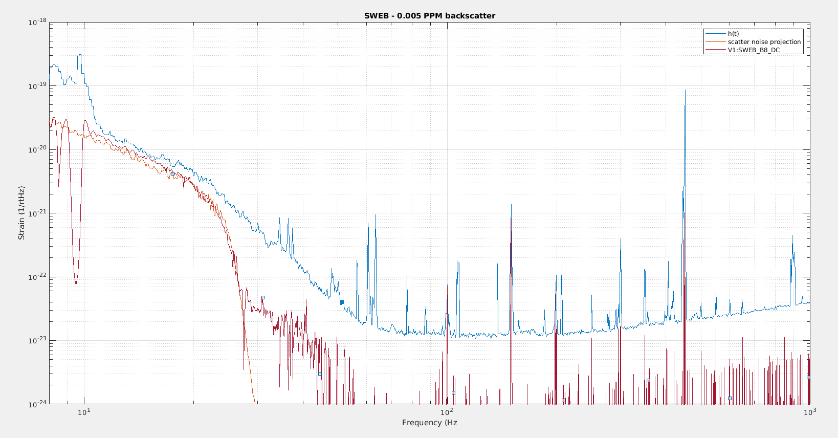
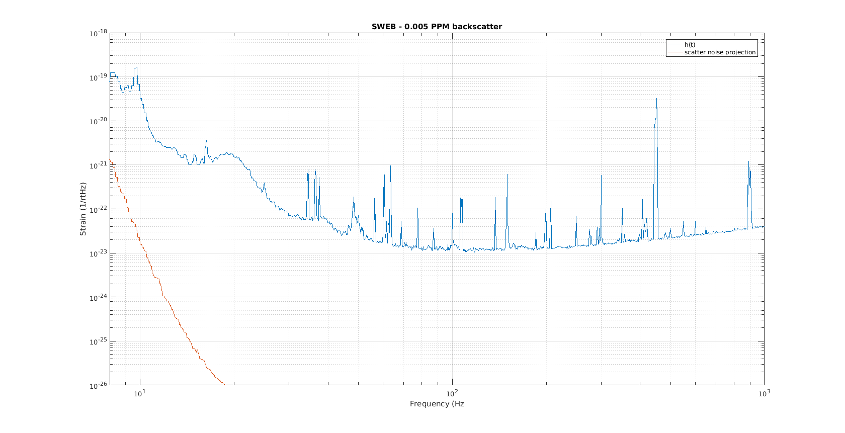
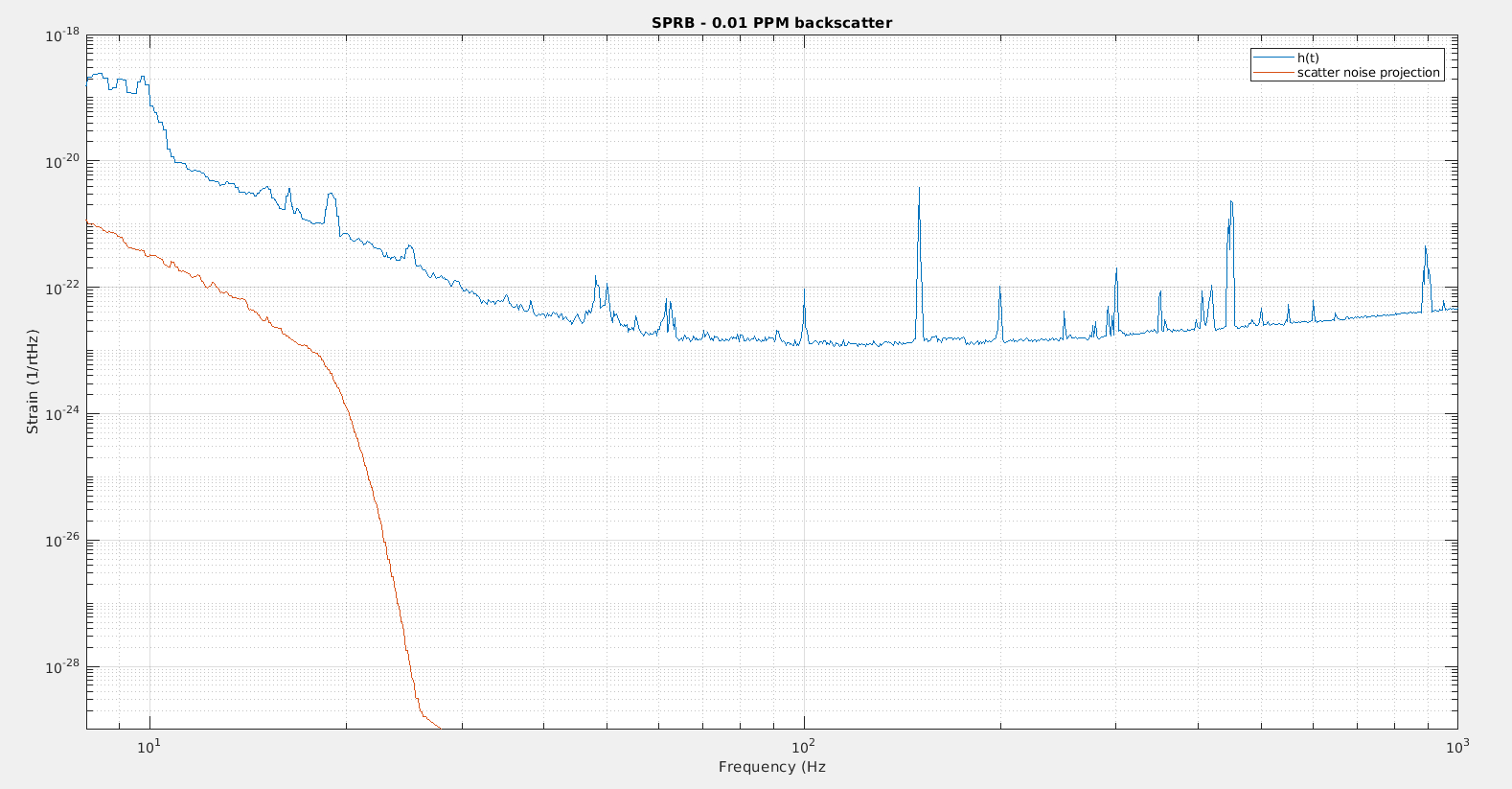
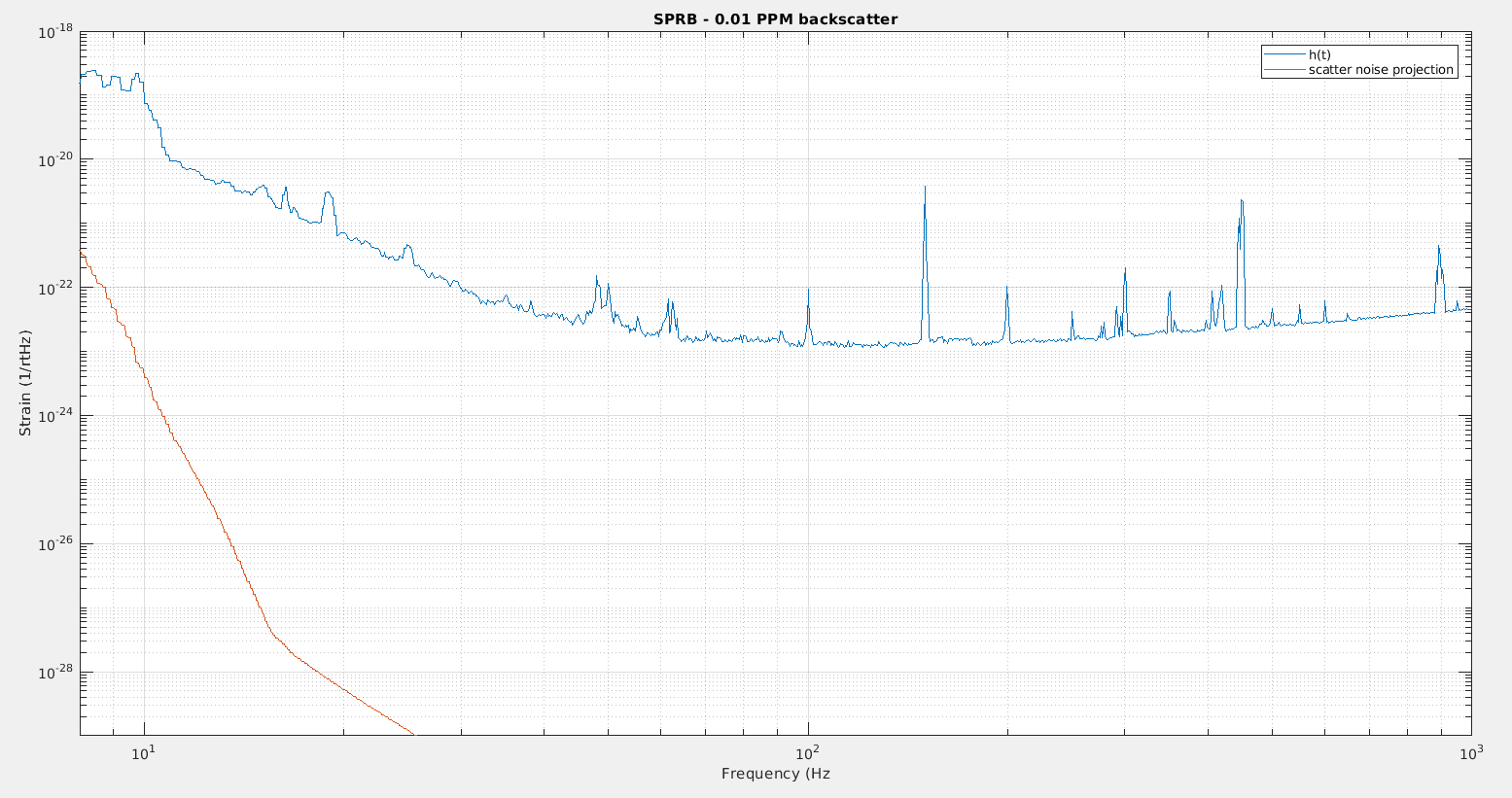
Figure 7. For SWEB (and SNEB) there are no recent injection (they are planned for the October break). But for SWEB nature provides injections whenever the sea is stormy. Taking here data from April 4th 2019 at 7:10 UTC. The scattering is not sufficient to dominate h(t) raw (before B7, B8 subtraction), but the scattered light coupling can be measured directly by measuring the transfer function between B8 and h(t), and using it to project the B8_DC spectrum. This is shown in dark red on the figure. In light red the projection using the modeled transfer function and the fringe wrapped motion of SWEB is shown. It matches very well if a back scatter of 0.005 PPM is assumed.


