Yesterday evening the successful lock acquisition was achieved by misaligning SR TY by ~2urad in DRMI before continuing the lock acquisition. This is in fact the standard lock procedure during the science run as SR TY is misaligned by 2urad in LN3, and SR is not realigned in DRMI. It only gets realigned in CARM NULL 1F, and the misaligned again at the LN2->LN3 transition.
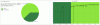
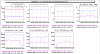
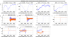
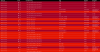
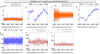
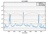
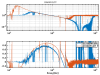
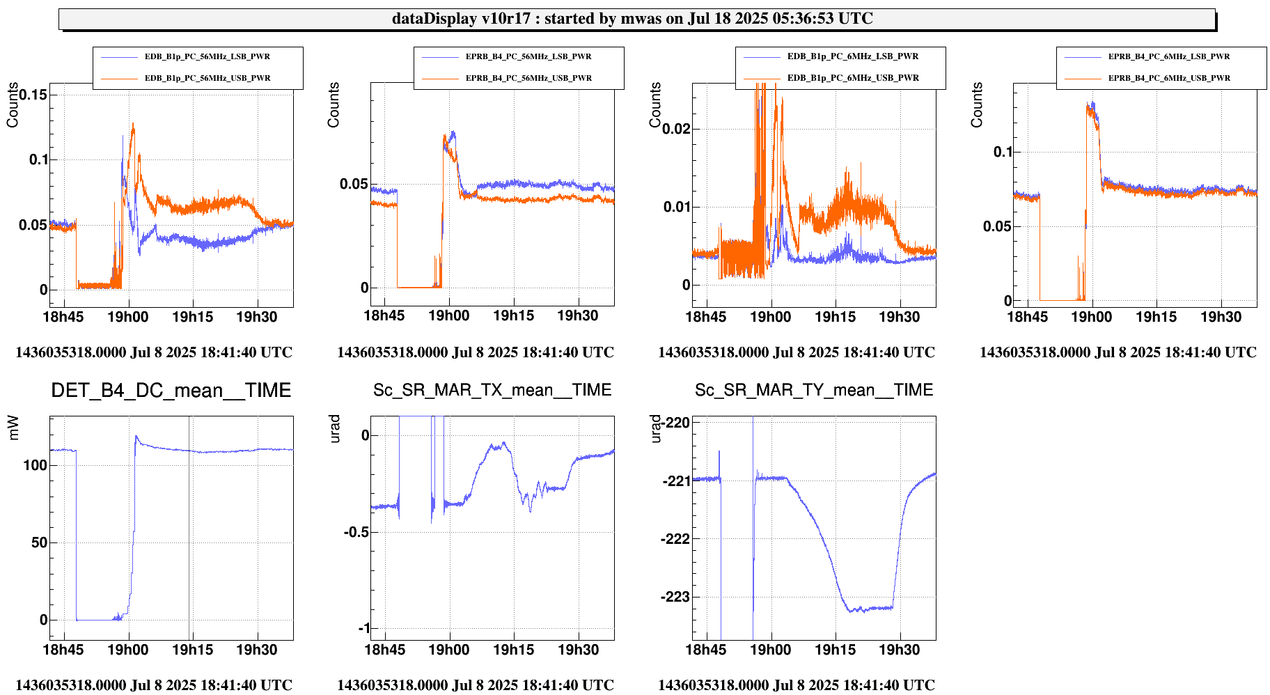
Figure 1 shows a standard lock acquisition last week when there was lots of unlocks from LN3 caused by BS F0 glitches. SR TY is at -221 at the beginning, then comes back to that position after the unlock (where SR is misaligned to remove it from the CITF), the ones the interferometer reaches CARM NULL 1F SR TY progressively decreases to -223, and then finally at ~19:30 UTC it increases back to -221 during the LN2->LN3 transition
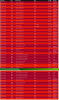
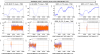
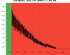
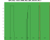
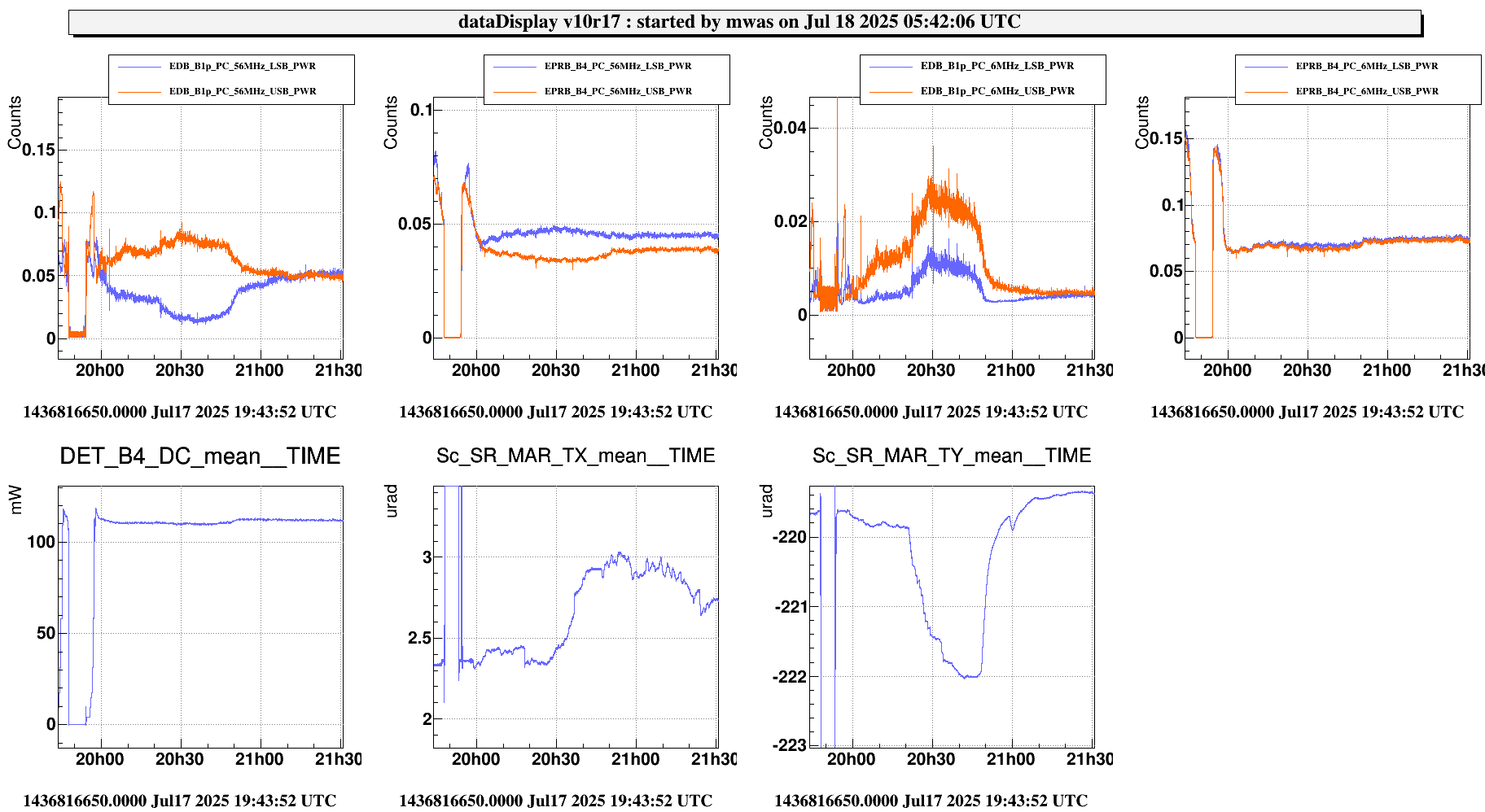
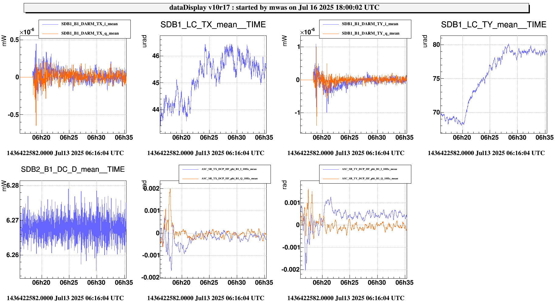
Figure 2 shows the successful lock acquisition of last night, it reproduces the same shaep of SR TY alignment. However the misalignment had to be done manually, using many manual steps of SR TY.
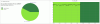
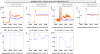
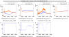
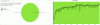
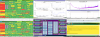
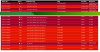
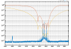
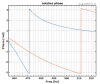
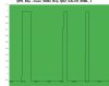
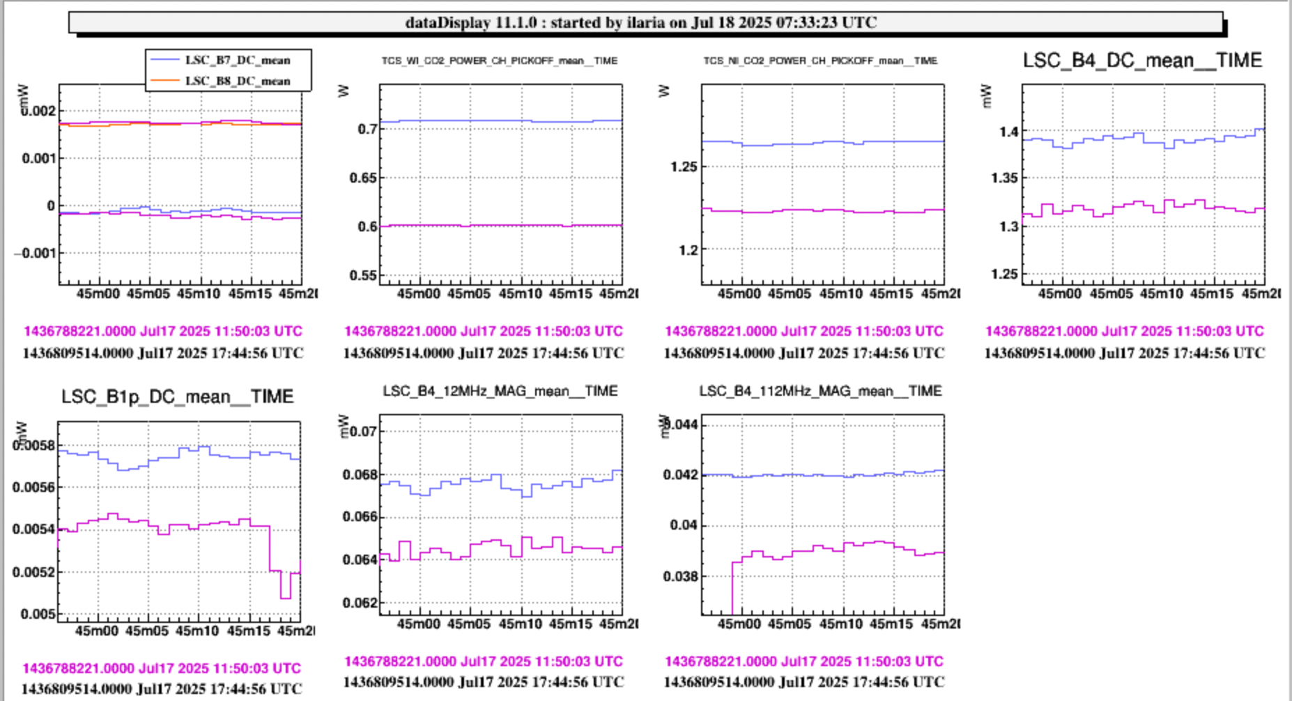
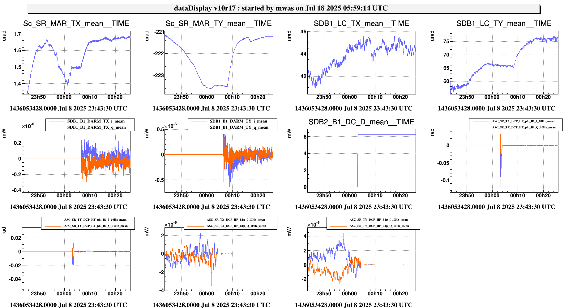
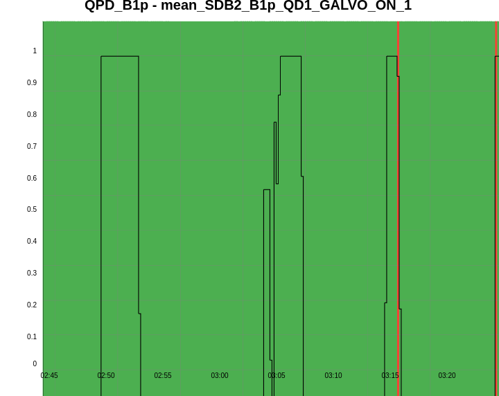
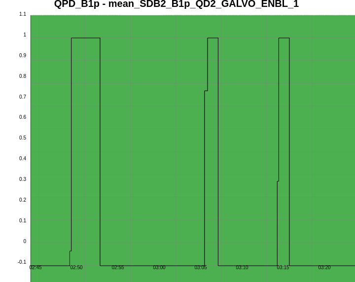
Figure 3 shows a normal lock acqusition, the SR TY DCP HF B1p I signal is away from zero and the moves to zero as SR TY moves from -221 to -223 in CARM NULL 1F. If I am not mistaken that is the error signal for the SR TY loop in CARM NULL 1F.
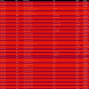
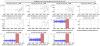
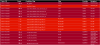
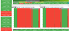
Figure 4 shows the same last night. There is no changes on SR TY DCP HF B1p I during the SR TY realingment in CARM NULL (transition from -220 to -222). This is not hidden by noise of the signal as the noise is +/-1e-9 peak to peak, while in figure 3 the transient is 3e-9.
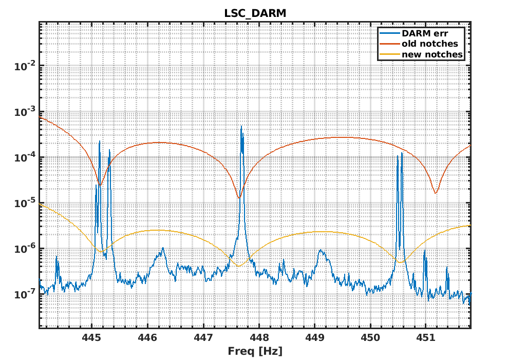
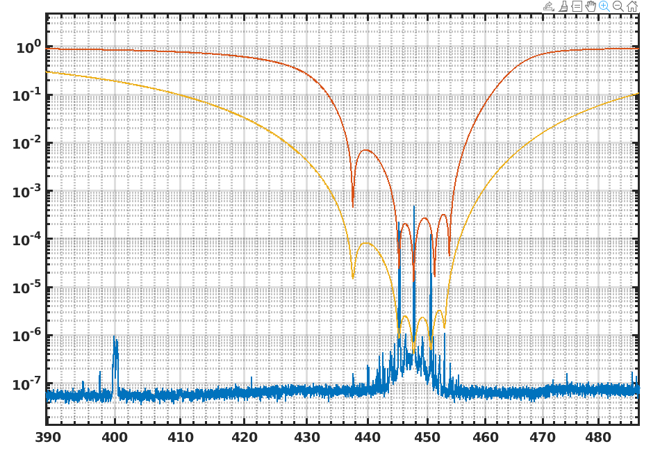
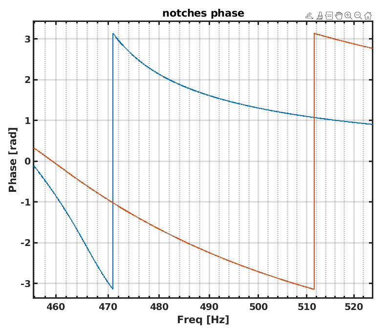
This is most likely due to the change in the notch of the violin modes https://logbook.virgo-gw.eu/virgo/?r=67311 . We should return to the standard notch filters of the violin modes, undo the changes in the DCP pole frequency calculation done in CARM NULL 1F, and check if the SR alignment signals are recovered.


